Matlab meets the steam tables
John Kitchin
A Matlab module for the steam tables is available for download at http://www.x-eng.com/XSteam_Matlab.htm. To do this example yourself, you need to download this zipfile and unzip it into your Matlab path. Today we will examine using this module for examining the Rankine power generation cycle, following example3.7-1 in Sandler's Thermodynamics book.
Problem statement: A Rankine cycle operates using steam with the condenser at 100 degC, a pressure of 3.0 MPa and temperature of 600 degC in the boiler. Assuming the compressor and turbine operate reversibly, estimate the efficiency of the cycle.
We will use the XSteam module to compute the required properties. There is only one function in XSteam, which takes a string and one or two arguments. The string specifies which subfunction to use.
We will use these functions from the module.
Contents
psat_T Saturation pressure (bar) at a specific T in degC
sL_T   Entropy (kJ/kg/K) of saturated liquid at T(degC)
hL_T   Enthalpy (kJ/kg)of saturated liquid at T(degC)
vL_T   Saturated liquid volume (m^3/kg)
T_ps   steam Temperature (degC) for a given pressure (bar) and entropy (kJ/kg/K)
h_pt   steam enthalpy (kJ/kg) at a given pressure (bar) and temperature (degC)
s_pt   steam entropy (kJ/kg/K) at a given pressure (bar) and temperature (degC)
We will use the cmu.units package to keep track of the units. Remember that the units package internally stores units in terms of base units, so to get a pressure in bar, we use the syntax P/u.bar, which is a dimensionless number with a magnitude equal to the number of bar.
clear all; clc; close all
u = cmu.units;
Starting point in the Rankine cycle in condenser.
we have saturated liquid here, and we get the thermodynamic properties for the given temperature.
T1 = 100;
P1 = XSteam('psat_T',T1)*u.bar;
s1 = XSteam('sL_T', T1)*u.kJ/u.kg/u.K;
h1 = XSteam('hL_t', T1)*u.kJ/u.kg;
v1 = XSteam('vL_T', T1)*u.m^3/u.kg;
isentropic compression of liquid to point 2
The final pressure is given, and we need to compute the new temperatures, and enthalpy.
P2 = 3*u.MPa;
s2 = s1;
T2 = XSteam('T_ps',P2/u.bar, s1/(u.kJ/u.kg/u.K));
h2 = XSteam('h_pt', P2/u.bar,T2)*u.kJ/u.kg;
WdotP = v1*(P2-P1);
fprintf('the compressor work is: %s\n', WdotP.as(u.kJ/u.kg,'%1.2f'))
the compressor work is: 3.02*kJ/kg
isobaric heating to T3 in Boiler where we make steam
T3 = 600;
P3 = P2;
h3 = XSteam('h_pt', P3/u.bar, T3)*u.kJ/u.kg;
s3 = XSteam('s_pt', P3/u.bar, T3)*u.kJ/u.kg/u.K;
Qb = h3 - h2;
fprintf('the boiler heat duty is: %s\n', Qb.as(u.kJ/u.kg,'%1.2f'))
the boiler heat duty is: 3260.68*kJ/kg
isentropic expansion through turbine to point 4
Still steam
T4 = XSteam('T_ps',P1/u.bar, s3/(u.kJ/u.kg/u.K));
h4 = XSteam('h_pt', P1/u.bar, T4)*u.kJ/u.kg;
s4 = s3;
Qc = h4 - h1;
fprintf('the condenser heat duty is: %s\n', Qc.as(u.kJ/u.kg,'%1.2f'))
the condenser heat duty is: 2316.99*kJ/kg
This heat flow is not counted against the overall efficiency. Presumably a heat exchanger can do this cooling against the cooler environment, so only heat exchange fluid pumping costs would be incurred.
to get from point 4 to point 1
WdotTurbine = h4 - h3;
fprintf('the turbine work is: %s\n', WdotTurbine.as(u.kJ/u.kg,'%1.2f'))
the turbine work is: -946.72*kJ/kg
efficiency
This is a ratio of the work put in to make the steam, and the net work obtained from the turbine. The answer here agrees with the efficiency calculated in Sandler on page 135.
eta = -(WdotTurbine - WdotP)/Qb

fprintf('the overall efficiency is %1.0f%%\n', (eta*100))
eta =

   0.291271696419079

the overall efficiency is 29%
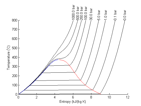
Entropy-temperature chart
The XSteam module makes it pretty easy to generate figures of the steam tables. Here we generate an entropy-Temperature graph.
T = linspace(0,800,200);
figure; hold on
for P = [0.01 0.1 1 5 30 100 250 500 1000]
S = arrayfun(@(t) XSteam('s_PT',P,t),T);
plot(S,T,'k-')
text(S(end),T(end),sprintf('%1.1f bar',P),'rotation',90)
end
set(gca,'Position',[0.13 0.11 0.775 0.7])
svap = arrayfun(@(t) XSteam('sV_T',t),T);
sliq = arrayfun(@(t) XSteam('sL_T',t),T);
plot(svap,T,'r-')
plot(sliq,T,'b-')
xlabel('Entropy (kJ/(kg K)')
ylabel('Temperature (^\circC)')
Plot Path
The path from 1 to 2 is isentropic, and has a small T change.
plot([s1 s2]/(u.kJ/u.kg/u.K),...
[T1 T2],'ro ','markersize',8,'markerfacecolor','r')
T23 = linspace(T2, T3);
S23 = arrayfun(@(t) XSteam('s_PT',P2/u.bar,t),T23);
plot(S23,T23,'b-','linewidth',4)
plot([s3 s4]/(u.kJ/u.kg/u.K),...
[T3 T4],'g-','linewidth',4)
T41 = linspace(T4,T1-0.01);
S41 = arrayfun(@(t) XSteam('s_PT',P1/u.bar,t),T41);
plot(S41,T41,'r-','linewidth',4)
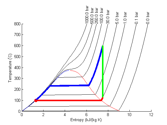
Note steps 1 and 2 are very close together on this graph and hard to see.
Summary
This was an interesting exercise. On one hand, the tedium of interpolating the steam tables is gone. On the other hand, you still have to know exactly what to ask for to get an answer that is correct. The XSteam interface is a little clunky, and takes some getting used to. It would be nice if it was vectorized to avoid the arrayfun calls.
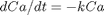 for multiple values of
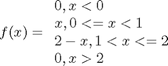
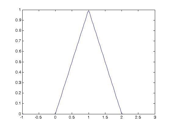
  . Here we use a trick to pass a parameter to an ODE through the initial conditions. We expand the ode function definition to include this parameter, and set its derivative to zero, effectively making it a constant.
 value decays faster.
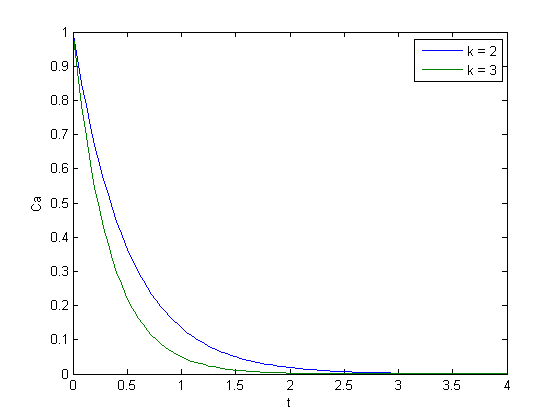


 , so that at
  we have a simpler problem we know how to solve, and at
  we have the original set of equations. Then, we derive a set of ODEs on how the solution changes with
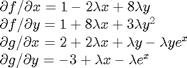
  , which has two roots,
  and
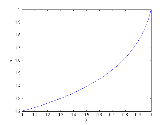
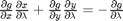
and  . We will use the method of continuity to solve this equation to illustrate a few ideas. First, we introduce a new variable
  . For example, we could write
  . Now, when
  , with the solution
  . The question now is, how does
  change as
  changes with
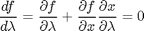
 and
and  analytically from our equation and solve for
  as
as
 and
and  .
.
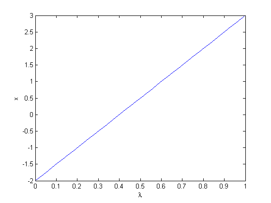
 into the equations in another way. We could try:
  , but this leads to an ODE that is singular at the initial starting point. Another approach is
  , but now the solution at
  is imaginary, and we don't have a way to integrate that! What we can do instead is add and subtract a number like this:
  . Now at
  , and we already know that
  is a solution. So, we create our ODE on
  with initial condition
  .
.
 , you find that 2 is a root, and learn nothing new. You could choose other values to add, e.g., if you chose to add and subtract 16, then you would find that one starting point leads to one root, and the other starting point leads to the other root. This method does not solve all problems associated with nonlinear root solving, namely, how many roots are there, and which one is "best"? But it does give a way to solve an equation where you have no idea what an initial guess should be. You can see, however, that just like you can get different answers from different initial guesses, here you can get different answers by setting up the equations differently.

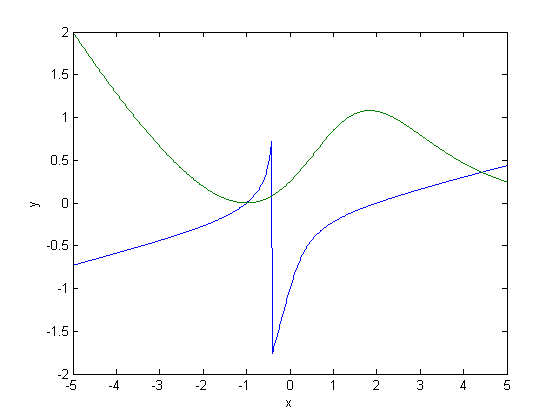
 , which will vary from 0 to 1. at
  we will have a simpler equation, preferrably a linear one, which can be solved, which can be analytically solved. At
  , we have the original equations. Then, we create a system of differential equations that start at this solution, and integrate from


 . Why do we do that? The solution, (x,y) will be a function of
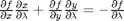
 and
and  . You can use Cramer's rule to solve for these to yield:
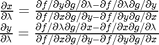
 and
and  , with the initial conditions at
  which is the solution of the simpler linear equations, and integrate to
  , which is the final solution of the original equations!
 , which is the solution to the original equations.
 starting point, so it is possible to miss solutions this way. For problems with lots of variables, this would be a good approach if you can identify the easy problem.