Yet another way to parameterize an ODE

John Kitchin

In posts Post 1108 and Post 1130 we examined two ways to parameterize an ODE. In those methods, we either used an anonymous function to parameterize an ode function, or we used a nested function that used variables from the shared workspace.

We want a convenient way to solve 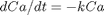for multiple values of . Here we use a trick to pass a parameter to an ODE through the initial conditions. We expand the ode function definition to include this parameter, and set its derivative to zero, effectively making it a constant.

function main

tspan = linspace(0,4);
Ca0 = 1;
k1 = 2;

init = [Ca0 k1]; % include k1 as an initial condition

[t1 C1] = ode45(@odefunc, tspan, init);

Now we can easily change the value of k like this

k2 = 3;
init = [Ca0 k2];

[t2 C2] = ode45(@odefunc, tspan, init);

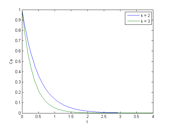
And plot both curves together. You can see the larger value decays faster.

plot(t1,C1(:,1),t2,C2(:,1))
xlabel('t')
ylabel('Ca')
legend 'k = 2' 'k = 3'

I don't think this is a very elegant way to pass parameters around compared to the previous methods in Post 1108 and Post 1130 , but it nicely illustrates that there is more than one way to do it. And who knows, maybe it will be useful in some other context one day!

'done'

ans =

done

function dCdt = odefunc(t,C)

dCa/dt = -k*Ca

C is a vector containing Ca in the first element, and k in the second element. This function is a subfunction, not a nested function.

Ca = C(1);
k = C(2);

dCadt = -k*Ca;
dkdt = 0; % this is the parameter we are passing in. it is a constant.

dCdt = [dCadt; dkdt];

% categories: ODEs

Published with MATLAB® 7.12