Matlab in Chemical Engineering at CMU

Method of continuity for solving nonlinear equations - Part II

November 02, 2011 at 01:25 PM | categories: nonlinear algebra | View Comments

Method of continuity for solving nonlinear equations - Part II

John Kitchin

clear all; close all; clc

Yesterday in Post 1324 we looked at a way to solve nonlinear equations that takes away some of the burden of initial guess generation. The idea was to reformulate the equations with a new variable $\lambda$ , so that at $\lambda=0$ we have a simpler problem we know how to solve, and at $\lambda=1$ we have the original set of equations. Then, we derive a set of ODEs on how the solution changes with $\lambda$ , and solve them.

Today we look at a simpler example and explain a little more about what is going on. Consider the equation: 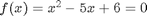$f(x) = x^2 - 5x + 6 = 0$ , which has two roots, $x=2$ and $x=3$ . We will use the method of continuity to solve this equation to illustrate a few ideas. First, we introduce a new variable $\lambda$ as: $f(x; \lambda) = 0$ . For example, we could write $f(x;\lambda) = \lambda x^2 - 5x + 6 = 0$ . Now, when $\lambda=0$ , we hve the simpler equation $- 5x + 6 = 0$ , with the solution $x=6/5$ . The question now is, how does $x$ change as $\lambda$ changes? We get that from the total derivative of how $f(x,\lambda)$ changes with $\lambda$ . The total derivative is:

$\frac{df}{d\lambda} = \frac{\partial f}{\partial \lambda} + \frac{\partial f}{\partial x}\frac{\partial x}{\partial \lambda}=0$

We can calculate two of those quantities: $\frac{\partial f}{\partial \lambda}$ and $\frac{\partial f}{\partial x}$ analytically from our equation and solve for $\frac{\partial x}{\partial \lambda}$ as

$\frac{\partial x}{\partial \lambda} = -\frac{\partial f}{\partial \lambda}/\frac{\partial f}{\partial x}$

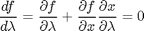
That defines an ordinary differential equation that we can solve by integrating from $\lambda=0$ where we know the solution to $\lambda=1$ which is the solution to the real problem. For this problem: $\frac{\partial f}{\partial \lambda}=x^2$ and $\frac{\partial f}{\partial x}=-5 + 2\lambda x$ .

dxdL = @(lambda,x) -x^2/(-5 + 2*lambda*x);

[L,x] = ode45(dxdL,[0 1], 6/5);

plot(L,x)
xlabel('\lambda')
ylabel('x')
fprintf('One solution is at x = %1.2f\n', x(end))

One solution is at x = 2.00

We found one solution at x=2. What about the other solution? To get that we have to introduce $\lambda$ into the equations in another way. We could try: $f(x;\lambda) = x^2 + \lambda(-5x + 6)$ , but this leads to an ODE that is singular at the initial starting point. Another approach is $f(x;\lambda) = x^2 + 6 + \lambda(-5x)$ , but now the solution at $\lambda=0$ is imaginary, and we don't have a way to integrate that! What we can do instead is add and subtract a number like this: $f(x;\lambda) = x^2 - 4 + \lambda(-5x + 6 + 4)$ . Now at $\lambda=0$ , we have a simple equation with roots at $\pm 2$ , and we already know that $x=2$ is a solution. So, we create our ODE on $dx/d\lambda$ with initial condition $x(0) = -2$ .

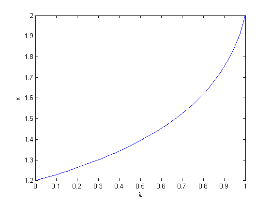
dxdL = @(lambda,x) (5*x-10)/(2*x-5*lambda);

[L,x] = ode45(dxdL,[0 1], -2);
plot(L,x)
xlabel('\lambda')
ylabel('x')
fprintf('One solution is at x = %1.2f\n', x(end))

One solution is at x = 3.00

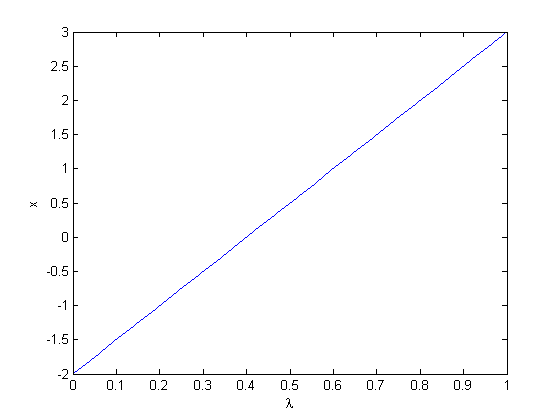
Now we have the other solution. Note if you choose the other root, $x=2$ , you find that 2 is a root, and learn nothing new. You could choose other values to add, e.g., if you chose to add and subtract 16, then you would find that one starting point leads to one root, and the other starting point leads to the other root. This method does not solve all problems associated with nonlinear root solving, namely, how many roots are there, and which one is "best"? But it does give a way to solve an equation where you have no idea what an initial guess should be. You can see, however, that just like you can get different answers from different initial guesses, here you can get different answers by setting up the equations differently.

% categories: Nonlinear algebra
% tags: math