Water gas shift equilibria via the NIST Webbook
December 13, 2011 at 01:49 AM | categories: miscellaneous, nonlinear algebra | View Comments
Water gas shift equilibria via the NIST Webbook
John Kitchin
The NIST webbook provides parameterized models of the enthalpy, entropy and heat capacity of many molecules. In this example, we will examine how to use these to compute the equilibrium constant for the water gas shift reaction  in the temperature range of 500K to 1000K.
Parameters are provided for:
Contents
 and
and 
   Cp = heat capacity (J/mol*K)
   H° = standard enthalpy (kJ/mol)
   S° = standard entropy (J/mol*K)
with models in the form: 


where  , and
, and  is the temperature in Kelvin. We can use this data to calculate equilibrium constants in the following manner. First, we have heats of formation at standard state for each compound; for elements, these are zero by definition, and for non-elements, they have values available from the NIST webbook. There are also values for the absolute entropy at standard state. Then, we have an expression for the change in enthalpy from standard state as defined above, as well as the absolute entropy. From these we can derive the reaction enthalpy, free energy and entropy at standard state, as well as at other temperatures.
We will examine the water gas shift enthalpy, free energy and equilibrium constant from 500K to 1000K, and finally compute the equilibrium composition of a gas feed containing 5 atm of CO and H2 at 1000K.
close all; clear all; clc;

T = linspace(500,1000); % degrees K
t = T/1000;
Setup equations for each species
First we enter in the parameters and compute the enthalpy and entropy for each species.
Hydrogen
% T = 298-1000K valid temperature range
A =  33.066178;
B = -11.363417;
C =  11.432816;
D = -2.772874;
E = -0.158558;
F = -9.980797;
G =  172.707974;
H =  0.0;

Hf_29815_H2 = 0.0; % kJ/mol
S_29815_H2 = 130.68; % J/mol/K

dH_H2 = A*t + B*t.^2/2 + C*t.^3/3 + D*t.^4/4 - E./t + F - H;
S_H2 = (A*log(t) + B*t + C*t.^2/2 + D*t.^3/3 - E./(2*t.^2) + G);
H2O
link Note these parameters limit the temperature range we can examine, as these parameters are not valid below 500K. There is another set of parameters for lower temperatures, but we do not consider them here.
% 500-1700 K valid temperature range
A =   30.09200;
B =   6.832514;
C =   6.793435;
D =  -2.534480;
E =   0.082139;
F =  -250.8810;
G =   223.3967;
H =  -241.8264;

Hf_29815_H2O = -241.83; %this is Hf.
S_29815_H2O = 188.84;

dH_H2O = A*t + B*t.^2/2 + C*t.^3/3 + D*t.^4/4 - E./t + F - H;
S_H2O = (A*log(t) + B*t + C*t.^2/2 + D*t.^3/3 - E./(2*t.^2) + G);
CO
% 298. - 1300K valid temperature range
A =   25.56759;
B =   6.096130;
C =   4.054656;
D =  -2.671301;
E =   0.131021;
F =  -118.0089;
G =   227.3665;
H = -110.5271;

Hf_29815_CO = -110.53; %this is Hf kJ/mol.
S_29815_CO = 197.66;

dH_CO = A*t + B*t.^2/2 + C*t.^3/3 + D*t.^4/4 - E./t + F - H;
S_CO = (A*log(t) + B*t + C*t.^2/2 + D*t.^3/3 - E./(2*t.^2) + G);
CO2
% 298. - 1200.K valid temperature range
A =   24.99735;
B =   55.18696;
C =  -33.69137;
D =   7.948387;
E =  -0.136638;
F =  -403.6075;
G =   228.2431;
H =  -393.5224;

Hf_29815_CO2 = -393.51; %this is Hf.
S_29815_CO2 = 213.79;

dH_CO2 = A*t + B*t.^2/2 + C*t.^3/3 + D*t.^4/4 - E./t + F - H;
S_CO2 = (A*log(t) + B*t + C*t.^2/2 + D*t.^3/3 - E./(2*t.^2) + G);
Standard state heat of reaction
We compute the enthalpy and free energy of reaction at 298.15 K for the following reaction  .
.
Hrxn_29815 = Hf_29815_CO2 + Hf_29815_H2 - Hf_29815_CO - Hf_29815_H2O;
Srxn_29815 = S_29815_CO2 + S_29815_H2 - S_29815_CO - S_29815_H2O;
Grxn_29815 = Hrxn_29815 - 298.15*(Srxn_29815)/1000;

sprintf('deltaH = %1.2f',Hrxn_29815)
sprintf('deltaG = %1.2f',Grxn_29815)
ans =

deltaH = -41.15


ans =

deltaG = -28.62
Correcting  and
and 
we have to correct for temperature change away from standard state. We only correct the enthalpy for this temperature change. The correction looks like this:

Where  are the stoichiometric coefficients of each species, with appropriate sign for reactants and products, and
  is precisely what is calculated for each species with the equations
Hrxn = Hrxn_29815 + dH_CO2 + dH_H2 - dH_CO - dH_H2O;
The entropy is on an absolute scale, so we directly calculate entropy at each temperature. Recall that H is in kJ/mol and S is in J/mol/K, so we divide S by 1000 to make the units match.
Grxn = Hrxn - T.*(S_CO2 + S_H2 - S_CO - S_H2O)/1000;
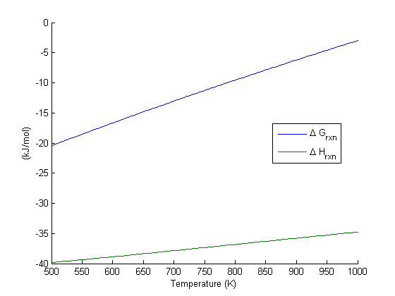
Plot how the  varies with temperature
over this temperature range the reaction is exothermic, although near 1000K it is just barely exothermic. At higher temperatures we expect the reaction to become endothermic.
figure; hold all
plot(T,Grxn)
plot(T,Hrxn)
xlabel('Temperature (K)')
ylabel('(kJ/mol)')
legend('\Delta G_{rxn}', '\Delta H_{rxn}', 'location','best')
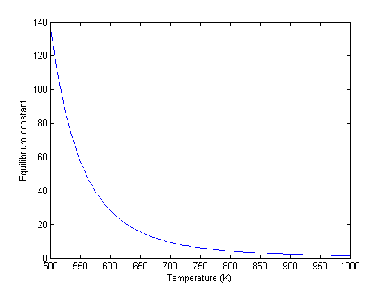
Equilibrium constant calculation
Note the equilibrium constant starts out high, i.e. strongly favoring the formation of products, but drops very quicky with increasing temperature.
R = 8.314e-3; %kJ/mol/K
K = exp(-Grxn/R./T);

figure
plot(T,K)
xlim([500 1000])
xlabel('Temperature (K)')
ylabel('Equilibrium constant')
Equilibrium yield of WGS
Now let's suppose we have a reactor with a feed of H2O and CO at 10atm at 1000K. What is the equilibrium yield of H2? Let  be the extent of reaction, so that
  . For reactants,
  is negative, and for products, is positive. We have to solve for the extent of reaction that satisfies the equilibrium condition.
A = CO
B = H2O
C = H2
D = CO2
Pa0 = 5; Pb0 = 5; Pc0 = 0; Pd0 = 0;  % pressure in atm
R = 0.082;
Temperature = 1000;

% we can estimate the equilibrium like this. We could also calculate it
% using the equations above, but we would have to evaluate each term. Above
% we simple computed a vector of enthalpies, entropies, etc...
K_Temperature = interp1(T,K,Temperature);

% If we let X be fractional conversion then we have $C_A = C_{A0}(1-X)$,
% $C_B = C_{B0}-C_{A0}X$, $C_C = C_{C0}+C_{A0}X$, and $C_D =
% C_{D0}+C_{A0}X$. We also have $K(T) = (C_C C_D)/(C_A C_B)$, which finally
% reduces to $0 = K(T) - Xeq^2/(1-Xeq)^2$ under these conditions.

f = @(X) K_Temperature - X^2/(1-X)^2;

Xeq = fzero(f,[1e-3 0.999]);
sprintf('The equilibrium conversion for these feed conditions is: %1.2f',Xeq)
ans =

The equilibrium conversion for these feed conditions is: 0.55
Compute gas phase pressures of each species
Since there is no change in moles for this reaction, we can directly calculation the pressures from the equilibrium conversion and the initial pressure of gases. you can see there is a slightly higher pressure of H2 and CO2 than the reactants, consistent with the equilibrium constant of about 1.44 at 1000K. At a lower temperature there would be a much higher yield of the products. For example, at 550K the equilibrium constant is about 58, and the pressure of H2 is 4.4 atm due to a much higher equilibrium conversion of 0.88.
P_CO = Pa0*(1-Xeq)
P_H2O = Pa0*(1-Xeq)
P_H2 = Pa0*Xeq
P_CO2 = Pa0*Xeq
P_CO =

    2.2748


P_H2O =

    2.2748


P_H2 =

    2.7252


P_CO2 =

    2.7252
Compare the equilibrium constants
We can compare the equilibrium constant from the Gibbs free energy and the one from the ratio of pressures. They should be the same!
K_Temperature
(P_CO2*P_H2)/(P_CO*P_H2O)
K_Temperature =

    1.4352


ans =

    1.4352
Summary
The NIST Webbook provides a plethora of data for computing thermodynamic properties. It is a little tedious to enter it all into Matlab, and a little tricky to use the data to estimate temperature dependent reaction energies. A limitation of the Webbook is that it does not tell you have the thermodynamic properties change with pressure. Luckily, those changes tend to be small.
% categories: Miscellaneous, nonlinear algebra
% tags: thermodynamics, reaction engineering
 , so that at
  we have a simpler problem we know how to solve, and at
  we have the original set of equations. Then, we derive a set of ODEs on how the solution changes with
  , which has two roots,
  and
and  . We will use the method of continuity to solve this equation to illustrate a few ideas. First, we introduce a new variable
  . For example, we could write
  . Now, when
  , with the solution
  . The question now is, how does
  change as
  changes with
 and
and  analytically from our equation and solve for
  as
as
 and
and  .
.
 into the equations in another way. We could try:
  , but this leads to an ODE that is singular at the initial starting point. Another approach is
  , but now the solution at
  is imaginary, and we don't have a way to integrate that! What we can do instead is add and subtract a number like this:
  . Now at
  , and we already know that
  is a solution. So, we create our ODE on
  with initial condition
  .
.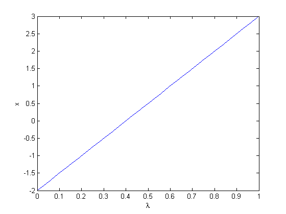
 , you find that 2 is a root, and learn nothing new. You could choose other values to add, e.g., if you chose to add and subtract 16, then you would find that one starting point leads to one root, and the other starting point leads to the other root. This method does not solve all problems associated with nonlinear root solving, namely, how many roots are there, and which one is "best"? But it does give a way to solve an equation where you have no idea what an initial guess should be. You can see, however, that just like you can get different answers from different initial guesses, here you can get different answers by setting up the equations differently.

 , which will vary from 0 to 1. at
  we will have a simpler equation, preferrably a linear one, which can be solved, which can be analytically solved. At
  , we have the original equations. Then, we create a system of differential equations that start at this solution, and integrate from


 . Why do we do that? The solution, (x,y) will be a function of
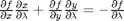
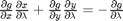
 and
and  . You can use Cramer's rule to solve for these to yield:
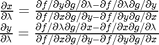
 and
and  , with the initial conditions at
  which is the solution of the simpler linear equations, and integrate to
  , which is the final solution of the original equations!
 , which is the solution to the original equations.
 starting point, so it is possible to miss solutions this way. For problems with lots of variables, this would be a good approach if you can identify the easy problem.
 . Unfortunately, the correlations for laminar flow and turbulent flow have different values at the transition that should occur at Re = 3000. This discontinuity can cause a lot of problems for numerical solvers that rely on derivatives.
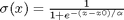 . The transition is centered on
  determines the width of the transition.
 and
and  we want to smoothly join, we do it like this:
  . There is no formal justification for this form of joining, it is simply a mathematical convenience to get a numerically smooth function. Other functions besides the sigmoid function could also be used, as long as they smoothly transition from 0 to 1, or from 1 to zero.
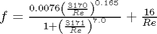 . Here we show the comparison with the approach used above. The friction factor differs slightly at high Re, becauase Morrison's is based on the Prandlt correlation, while the work here is based on the Nikuradse correlation. They are similar, but not the same.
 , and the corresponding pressure drop is given by
  . In these equations,
  is the fluid density,
  is the fluid velocity,
  is the pipe diameter, and
  is the Fanning friction factor. The average fluid velocity is given by
  .
. , which is a linear equation, and for turbulent flow (
 ) we have the implicit equation
 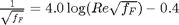 . Of course, we define
  where
where  is the viscosity of the fluid.
 and
and  where
where 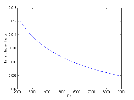
 that solves: $ \Delta p = \rho 2 f_F \frac{\Delta L v^2}{D}$. This is a nonlinear equation in