Calculating a bubble point pressure
September 16, 2011 at 01:38 AM | categories: nonlinear algebra | View Comments
Calculating a bubble point pressure
adapted from http://terpconnect.umd.edu/~nsw/ench250/bubpnt.htm
In Post 1060 we learned to read a datafile containing lots of Antoine coefficients into a database, and use the coefficients to estimate vapor pressure. Today, we use those coefficents to compute a bubble point pressure. You will need download antoine_database.mat if you haven't already run the previous example.
The bubble point is the temperature at which the sum of the component vapor pressures is equal to the the total pressure. This is where a bubble of vapor will first start forming, and the mixture starts to boil.
Consider an equimolar mixture of benzene, toluene, chloroform, acetone and methanol. Compute the bubble point at 760 mmHg, and the gas phase composition.
Contents
Load the parameter database
load antoine_database.mat
list the compounds
compounds = {'benzene' 'toluene' 'chloroform' 'acetone' 'methanol'}
n = numel(compounds); % we use this as a counter later.
compounds =

  Columns 1 through 4

    'benzene'    'toluene'    'chloroform'    'acetone'

  Column 5

    'methanol'
preallocate the vectors
for large problems it is more efficient to preallocate the vectors.
A = zeros(n,1); B = zeros(n,1); C = zeros(n,1);
Tmin = zeros(n,1); Tmax = zeros(n,1);
Now get the parameters for each compound
for i = 1:n
    c = database(compounds{i}); % c is a cell array
    % assign the parameters to the variables
    [A(i) B(i) C(i) Tmin(i) Tmax(i)] = c{:};
end
this is the equimolar, i.e. equal mole fractions
x = [0.2; 0.2; 0.2; 0.2; 0.2];
Given a T, we can compute the pressure of each species like this:
T = 67; % degC
P = 10.^(A-B./(T + C))
P =

  1.0e+003 *

    0.4984
    0.1822
    0.8983
    1.0815
    0.8379
note the pressure is a vector, one element for each species. To get the total pressure of the mixture, we use the sum command, and multiply each pure component vapor pressure by the mole fraction of that species.
sum(x.*P)
% This is less than 760 mmHg, so the Temperature is too low.
ans =

  699.6546
Solve for the bubble point
We will use fsolve to find the bubble point. We define a function that is equal to zero at teh bubble point. That function is the difference between the pressure at T, and 760 mmHg, the surrounding pressure.
Tguess = 67;
Ptotal = 760;
func = @(T) Ptotal - sum(x.*10.^(A-B./(T + C)));

T_bubble = fsolve(func,Tguess)

sprintf('The bubble point is %1.2f degC', T_bubble)
Equation solved.

fsolve completed because the vector of function values is near zero
as measured by the default value of the function tolerance, and
the problem appears regular as measured by the gradient.


T_bubble =

   69.4612


ans =

The bubble point is 69.46 degC
Let's double check the T_bubble is within the valid temperature ranges
if any(T_bubble < Tmin) | any(T_bubble > Tmax) % | is the "or" operator
    error('T_bubble out of range')
else
    sprintf('T_bubble is in range')
end
ans =

T_bubble is in range
Vapor composition
we use the formula y_i = x_i*P_i/P_T.
y = x.*10.^(A-B./(T_bubble + C))/Ptotal;

for i=1:n
    sprintf('y_%s = %1.3f',compounds{i},y(i))
end
ans =

y_benzene = 0.142


ans =

y_toluene = 0.053


ans =

y_chloroform = 0.255


ans =

y_acetone = 0.308


ans =

y_methanol = 0.242
Summary
we saved some typing effort by using the parameters from the database we read in before. We also used the vector math capability of matlab to do element by element processing, e.g. in line 44 and 58. This let us avoid doing some loop programming, or writing equations with 5 compounds in them!
% categories: nonlinear algebra
% tags: thermodynamics
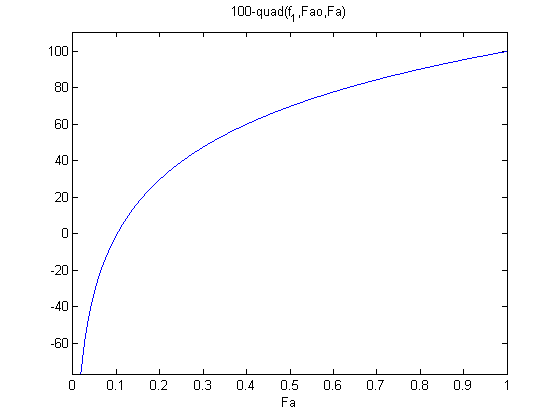
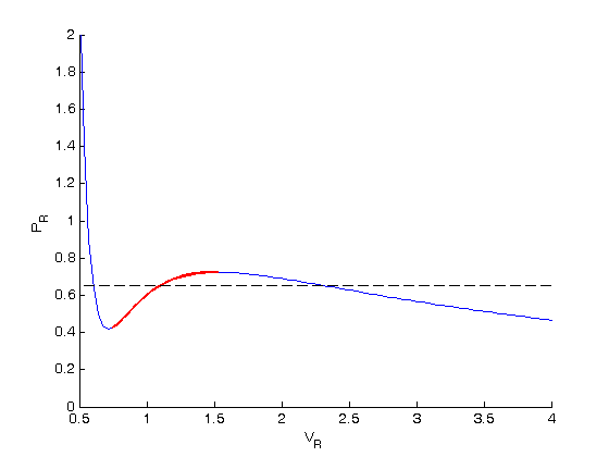
 , the isotherm fails to describe real materials, which phase separate into a liquid and gas in this region.
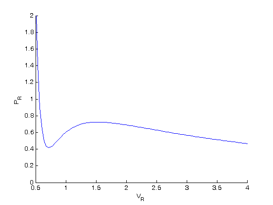
 . We use the coefficients t0 get the rooys like this.
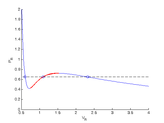
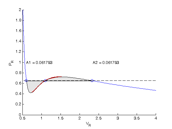
 . We use logical indexing to select the parts of the data that we want.
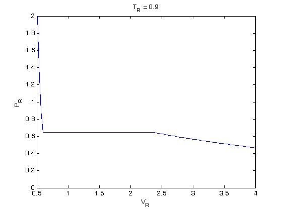
 . You could also compute the isotherm for other
  values.
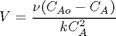
 where
where  is the rate law. Suppose we know the reactor volume is 100 L, the inlet molar flow of A is 1 mol/L, the volumetric flow is 10 L/min, and
  , with
  1/min. What is the exit molar flow rate? We need to solve the following equation: