The equal area method for the van der Waals equation

John Kitchin

Contents

Introduction

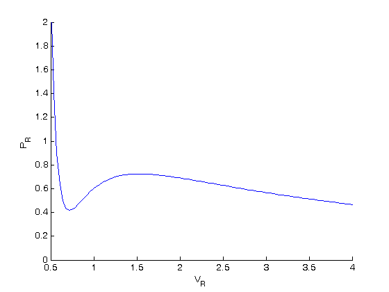
When a gas is below its Tc the van der Waal equation oscillates. In the portion of the isotherm where , the isotherm fails to describe real materials, which phase separate into a liquid and gas in this region.

Maxwell proposed to replace this region by a flat line, where the area above and below the curves are equal. Today, we examine how to identify where that line should be.

function maxwell_equal_area_2

clc; clear all; close all

Tr = 0.9; % A Tr below Tc:  Tr = T/Tc
% analytical equation for Pr. This is the reduced form of the van der Waal
% equation.
Prfh = @(Vr) 8/3*Tr./(Vr - 1/3) - 3./(Vr.^2);

Vr = linspace(0.5,4,100);   % vector of reduced volume
Pr = Prfh(Vr);              % vector of reduced pressure

Plot the vdW EOS

figure; hold all
plot(Vr,Pr)
ylim([0 2])
xlabel('V_R')
ylabel('P_R')

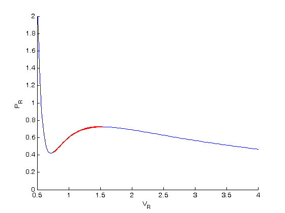
show unstable region

dPdV = cmu.der.derc(Vr, Pr);
plot(Vr(dPdV > 0),Pr(dPdV > 0),'r-','linewidth',2)

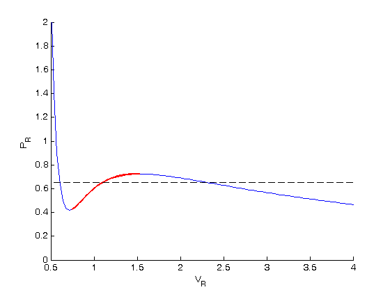
Idea behind Maxwell equal area principle

The idea is to pick a Pr and draw a line through the EOS. We want the areas between the line and EOS to be equal on each side of the middle intersection.

y = 0.65;  % Pr that defines the horizontal line
plot([0.5 4],[y y],'k--') % horizontal line

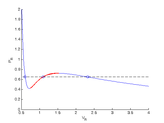
find three roots

To find the areas, we need to know where the intersection of the vdW eqn with the horizontal line. This is the same as asking what are the roots of the vdW equation at that Pr. We need all three intersections so we can integrate from the first root to the middle root, and then the middle root to the third root. We take advantage of the polynomial nature of the vdW equation, which allows us to use the roots command to get all the roots at once. The polynomial is . We use the coefficients t0 get the rooys like this.

vdWp = [1 -1/3*(1+8*Tr/y) 3/y -1/y];
v = sort(roots(vdWp))

v =

    0.6029
    1.0974
    2.3253

plot the roots

we want to make sure the roots are really the intersections with the line.

plot(v(1),y,'bo',v(2),y,'bo',v(3),y,'bo')

compute areas

for A1, we need the area under the line minus the area under the vdW curve. That is the area between the curves. For A2, we want the area under the vdW curve minus the area under the line. The area under the line between root 2 and root 1 is just the width (root2 - root1)*y

A1 = (v(2)-v(1))*y - quad(Prfh,v(1),v(2))
A2 = quad(Prfh,v(2),v(3)) - (v(3)-v(2))*y
% these areas are pretty close, and we could iterate to get them very
% close. or, we can use a solver to do this. To do that, we need to define
% a function that is equal to zero when the two areas are equal. See the
% equalArea function below.

Pr_equal_area = fzero(@equalArea, 0.65)

A1 =

    0.0632


A2 =

    0.0580


Pr_equal_area =

    0.6470

confirm the two areas are equal

y = Pr_equal_area;
equalArea(y) % this should be close to zero

ans =

  1.1102e-016

and we can compute the areas too

vdWp = [1 -1/3*(1+8*Tr/y) 3/y -1/y]
v = sort(roots(vdWp))
A1 = (v(2)-v(1))*y - quad(Prfh,v(1),v(2))
A2 = quad(Prfh,v(2),v(3)) - (v(3)-v(2))*y
% these areas are very close to each other.

vdWp =

    1.0000   -4.0428    4.6368   -1.5456


v =

    0.6034
    1.0905
    2.3488


A1 =

    0.0618


A2 =

    0.0618

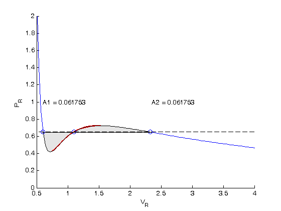
plot the areas that are equal

we want to show the areas that are equal by shading them.

xx = [v(1) Vr(Vr >= v(1) & Vr <= v(2)) v(2)];
yy = [Prfh(v(1)) Pr(Vr >= v(1) & Vr <= v(2)) Prfh(v(2))];
lightgray = [0.9 0.9 0.9];
fill(xx,yy,lightgray)

xx = [v(2) Vr(Vr >= v(2) & Vr <= v(3)) v(3)];
yy = [Prfh(v(2)) Pr(Vr >= v(2) & Vr <= v(3)) Prfh(v(3))];
fill(xx,yy,lightgray)
% and finally lets add text labels to the figure for what the areas are.
text(v(1),1,sprintf('A1 = %f',A1))
text(v(3),1,sprintf('A2 = %f',A2))

Finally, plot the isotherm

we want to replace the unstable region with the flat line that defines the equal areas. The roots are stored in the variable . We use logical indexing to select the parts of the data that we want.

figure
Vrf = [Vr(Vr <= v(1)) v(1)       v(3)       Vr(Vr>= v(3))];
Prf = [Pr(Vr <= v(1)) Prfh(v(1)) Prfh(v(3)) Pr(Vr>= v(3))];
plot(Vrf,Prf)
ylim([0 2])
xlabel('V_R')
ylabel('P_R')
title('T_R = 0.9')

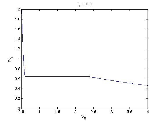
The flat line in this isotherm corresponds to a vapor-liquid equilibrium. This is the result for . You could also compute the isotherm for other values.

'done'

ans =

done

function Z = equalArea(y)
% compute A1 - A2 for Tr = 0.9.
Tr = 0.9;
vdWp = [1 -1/3*(1+8*Tr/y) 3/y -1/y];
v = sort(roots(vdWp));

Prfh = @(Vr) 8/3*Tr./(Vr - 1/3) - 3./(Vr.^2);
A1 = (v(2)-v(1))*y - quad(Prfh,v(1),v(2));
A2 = quad(Prfh,v(2),v(3)) - (v(3)-v(2))*y;

Z = A1 - A2;

% categories: Nonlinear algebra
% tags: thermodynamics

Published with MATLAB® 7.10