Method of continuity for nonlinear equation solving
November 01, 2011 at 07:53 PM | categories: nonlinear algebra | View Comments
Contents
Method of continuity for nonlinear equation solving
John Kitchin
Adapted from Perry's Chemical Engineers Handbook, 6th edition 2-63.
function main
We seek the solution to the following nonlinear equations:


f = @(x,y) 2 + x + y - x^2 + 8*x*y + y^3;
g = @(x,y) 1 + 2*x - 3*y + x^2 + x*y - y*exp(x);
In principle this is easy, we simply need some initial guesses. The challenge here is what would you guess? The equations are implicit, so it is not easy to graph them, but lets give it a shot, starting on the x range -5 to 5. The idea is set a value for x, and then solve for y in each equation
x = linspace(-5,5,500);
% at x = 0, we have 2 + y + y^3 = 0
fy = arrayfun(@(x) fzero(@(y) f(x,y), 0.1),x);
gy = arrayfun(@(x) fzero(@(y) g(x,y), 0),x);
plot(x,fy,x,gy)
xlabel('x')
ylabel('y')
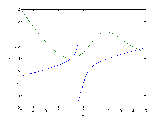
graphical solution
you can see there is a solution near x = -1, y = 0, because both functions equal zero there. We can even use that guess with fsolve. It is disappointly easy! But, keep in mind that in 3 or more dimensions, you cannot perform this visualization, and another method could be required.
f1 = @(X) [f(X(1),X(2)); g(X(1),X(2))];
fsolve(f1,[-1 0])
Equation solved at initial point.

fsolve completed because the vector of function values at the initial point
is near zero as measured by the default value of the function tolerance, and
the problem appears regular as measured by the gradient.


ans =

    -1     0
We explore a method that bypasses this problem today. The principle is to introduce a new variable,  , which will vary from 0 to 1. at
  we will have a simpler equation, preferrably a linear one, which can be solved, which can be analytically solved. At
  , we have the original equations. Then, we create a system of differential equations that start at this solution, and integrate from to , to recover the final solution.
We rewrite the equations as:


Now, at we have the simple linear equations:


x0 = [[1 1]; [2 -3]]\[-2; -1]
x0 =

   -1.4000
   -0.6000
Construct the system of ODEs
We form the system of ODEs by differentiating the new equations with respect to  . Why do we do that? The solution, (x,y) will be a function of . From calculus, you can show that:
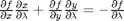
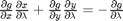
Now, solve this for  and
and  . You can use Cramer's rule to solve for these to yield:
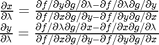
For this set of equations: 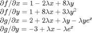
Now, we simply set up those two differential equations on  and
and  , with the initial conditions at
  which is the solution of the simpler linear equations, and integrate to
  , which is the final solution of the original equations!
    function dXdlambda = ode(lambda, X)
        x = X(1);
        y = X(2);

        pfpx = 1 - 2*lambda*x + 8*lambda*y;
        pfpy = 1 + 8*lambda*x + 3*lambda*y^2;
        pfplambda = -x^2+8*x*y+y^3;

        pgpx = 2 + 2*lambda*x + lambda*y - lambda*y*exp(x);
        pgpy = -3 + lambda*x - lambda*exp(x);
        pgplambda = x^2 + x*y -y*exp(x);

        dxdlambda = (pfpy*pgplambda - pfplambda*pgpy)/(pfpx*pgpy-pfpy*pgpx);
        dydlambda = (pfplambda*pgpx-pfpx*pgplambda)/(pfpx*pgpy-pfpy*pgpx);

        dXdlambda = [dxdlambda; dydlambda];
    end

[lambda X] = ode45(@ode,[0 1],x0);
the solution
The last X value corresponds to  , which is the solution to the original equations.
Xsol = X(end,:);
x = Xsol(1)
y = Xsol(2)
x =

   -1.0004


y =

 -2.9244e-004
evaluate solution
You can see the solution is somewhat approximate; the true solution is x = -1, y = 0. The approximation could be improved by lowering the tolerance on the ODE solver.
f(x,y)
g(x,y)
ans =

  7.1778e-004


ans =

    0.0013
Summary
This is a fair amount of work to get a solution! The idea is to solve a simple problem, and then gradually turn on the hard part by the lambda parameter. What happens if there are multiple solutions? The answer you finally get will depend on your  starting point, so it is possible to miss solutions this way. For problems with lots of variables, this would be a good approach if you can identify the easy problem.
end

% categories: Nonlinear algebra