Vectorized piecewise functions
November 06, 2011 at 12:13 AM | categories: miscellaneous | View Comments
Contents
Vectorized piecewise functions
John Kitchin
Occasionally we need to define piecewise functions, e.g.
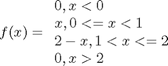
Today we examine a few ways to define a function like this.
function main
clear all; clc; close all
Use conditional statements in a function
    function y = f1(x)
        if x < 0
            y = 0;
        elseif x >= 0 & x < 1
            y = x;
        elseif x >= 1 & x < 2
            y = 2-x;
        else
            y = 0;
        end
    end
This works, but the function is not vectorized, i.e. f([-1 0 2 3]) does not evaluate at all, you get an error. You can get vectorized behavior by using the arrayfun function, or by writing your own loop. This doesn't fix all limitations, for example you cannot use the f1 function in the quad function to integrate it.
x = linspace(-1,3);
plot(x,arrayfun(@f1,x))
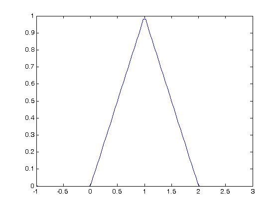
y = zeros(size(x));
for i=1:length(y)
    y(i) = f1(x(i));
end
plot(x,y)

Neither of those methods is convenient. It would be nicer if the function was vectorized, which would allow the direct notation f1([0 1 2 3 4]). A simple way to achieve this is through the use of logical arrays. We create logical arrays from comparison statements
x = linspace(-1,3,10)
x < 0
x =

  Columns 1 through 6

   -1.0000   -0.5556   -0.1111    0.3333    0.7778    1.2222

  Columns 7 through 10

    1.6667    2.1111    2.5556    3.0000


ans =

     1     1     1     0     0     0     0     0     0     0
x >= 0 & x < 1
ans =

     0     0     0     1     1     0     0     0     0     0
We can use the logical arrays as masks on functions; where the logical array is 1, the function value will be used, and where it is zero, the function value will not be used.
    function y = f2(x)
        % vectorized piecewise function
        % we start with zeros for all values of y(x)
        y = zeros(size(x));
        % now we add the functions, masked by the logical arrays.
        y = y + (x >= 0 & x < 1).*x;
        y = y + (x >= 1 & x < 2).*(2-x);
    end


x = linspace(-1,3);
plot(x,f2(x))

And now we can integrate it with quad!
quad(@f2,-1,3)
ans =

    1.0000
Third approach with Heaviside functions
The Heaviside function is defined to be zero for x less than some value, and 0.5 for x=0, and 1 for x >= 0. If you can live with y=0.5 for x=0, you can define a vectorized function in terms of Heaviside functions like this.
    function y = f3(x)
        y1 = (heaviside(x) - heaviside(x-1)).*x ; % first interval
        y2 = (heaviside(x-1) - heaviside(x-2)).*(2-x); % 2nd interval
        y = y1 + y2; % both intervals
    end

plot(x,f3(x))
quad(@f3,-1,3)
ans =

    1.0000

Summary
There are many ways to define piecewise functions, and vectorization is not always necessary. The advantages of vectorization are usually notational simplicity and speed; loops in Matlab are usually very slow compared to vectorized functions.
end

% categories: Miscellaneous
% tags: vectorization