Calculating a bubble point pressure

| categories: nonlinear algebra | View Comments

Calculating a bubble point pressure

Calculating a bubble point pressure

adapted from http://terpconnect.umd.edu/~nsw/ench250/bubpnt.htm

In Post 1060 we learned to read a datafile containing lots of Antoine coefficients into a database, and use the coefficients to estimate vapor pressure. Today, we use those coefficents to compute a bubble point pressure. You will need download antoine_database.mat if you haven't already run the previous example.

The bubble point is the temperature at which the sum of the component vapor pressures is equal to the the total pressure. This is where a bubble of vapor will first start forming, and the mixture starts to boil.

Consider an equimolar mixture of benzene, toluene, chloroform, acetone and methanol. Compute the bubble point at 760 mmHg, and the gas phase composition.

Contents

Load the parameter database

load antoine_database.mat

list the compounds

compounds = {'benzene' 'toluene' 'chloroform' 'acetone' 'methanol'}
n = numel(compounds); % we use this as a counter later.
compounds = 

  Columns 1 through 4

    'benzene'    'toluene'    'chloroform'    'acetone'

  Column 5

    'methanol'

preallocate the vectors

for large problems it is more efficient to preallocate the vectors.

A = zeros(n,1); B = zeros(n,1); C = zeros(n,1);
Tmin = zeros(n,1); Tmax = zeros(n,1);

Now get the parameters for each compound

for i = 1:n
    c = database(compounds{i}); % c is a cell array
    % assign the parameters to the variables
    [A(i) B(i) C(i) Tmin(i) Tmax(i)] = c{:};
end

this is the equimolar, i.e. equal mole fractions

x = [0.2; 0.2; 0.2; 0.2; 0.2];

Given a T, we can compute the pressure of each species like this:

T = 67; % degC
P = 10.^(A-B./(T + C))
P =

  1.0e+003 *

    0.4984
    0.1822
    0.8983
    1.0815
    0.8379

note the pressure is a vector, one element for each species. To get the total pressure of the mixture, we use the sum command, and multiply each pure component vapor pressure by the mole fraction of that species.

sum(x.*P)
% This is less than 760 mmHg, so the Temperature is too low.
ans =

  699.6546

Solve for the bubble point

We will use fsolve to find the bubble point. We define a function that is equal to zero at teh bubble point. That function is the difference between the pressure at T, and 760 mmHg, the surrounding pressure.

Tguess = 67;
Ptotal = 760;
func = @(T) Ptotal - sum(x.*10.^(A-B./(T + C)));

T_bubble = fsolve(func,Tguess)

sprintf('The bubble point is %1.2f degC', T_bubble)
Equation solved.

fsolve completed because the vector of function values is near zero
as measured by the default value of the function tolerance, and
the problem appears regular as measured by the gradient.


T_bubble =

   69.4612


ans =

The bubble point is 69.46 degC

Let's double check the T_bubble is within the valid temperature ranges

if any(T_bubble < Tmin) | any(T_bubble > Tmax) % | is the "or" operator
    error('T_bubble out of range')
else
    sprintf('T_bubble is in range')
end
ans =

T_bubble is in range

Vapor composition

we use the formula y_i = x_i*P_i/P_T.

y = x.*10.^(A-B./(T_bubble + C))/Ptotal;

for i=1:n
    sprintf('y_%s = %1.3f',compounds{i},y(i))
end
ans =

y_benzene = 0.142


ans =

y_toluene = 0.053


ans =

y_chloroform = 0.255


ans =

y_acetone = 0.308


ans =

y_methanol = 0.242

Summary

we saved some typing effort by using the parameters from the database we read in before. We also used the vector math capability of matlab to do element by element processing, e.g. in line 44 and 58. This let us avoid doing some loop programming, or writing equations with 5 compounds in them!

% categories: nonlinear algebra
% tags: thermodynamics
Read and Post Comments

The equal area method for the van der Waals equation

| categories: nonlinear algebra | View Comments

The equal area method for the van der Waals equation

The equal area method for the van der Waals equation

John Kitchin

Contents

Introduction

When a gas is below its Tc the van der Waal equation oscillates. In the portion of the isotherm where $\partial P_R/\partial V_r > 0$, the isotherm fails to describe real materials, which phase separate into a liquid and gas in this region.
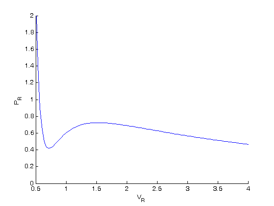
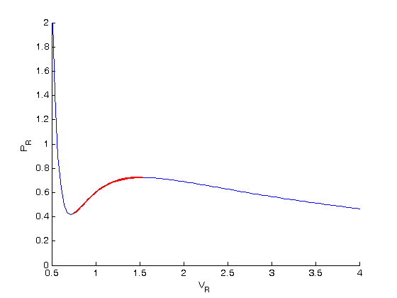
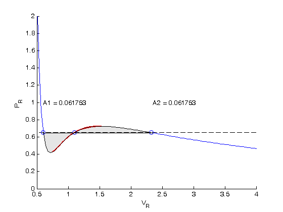
Maxwell proposed to replace this region by a flat line, where the area above and below the curves are equal. Today, we examine how to identify where that line should be.

function maxwell_equal_area_2
clc; clear all; close all

Tr = 0.9; % A Tr below Tc:  Tr = T/Tc
% analytical equation for Pr. This is the reduced form of the van der Waal
% equation.
Prfh = @(Vr) 8/3*Tr./(Vr - 1/3) - 3./(Vr.^2);

Vr = linspace(0.5,4,100);   % vector of reduced volume
Pr = Prfh(Vr);              % vector of reduced pressure

Plot the vdW EOS

figure; hold all
plot(Vr,Pr)
ylim([0 2])
xlabel('V_R')
ylabel('P_R')

show unstable region

dPdV = cmu.der.derc(Vr, Pr);
plot(Vr(dPdV > 0),Pr(dPdV > 0),'r-','linewidth',2)

Idea behind Maxwell equal area principle

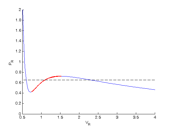
The idea is to pick a Pr and draw a line through the EOS. We want the areas between the line and EOS to be equal on each side of the middle intersection.

y = 0.65;  % Pr that defines the horizontal line
plot([0.5 4],[y y],'k--') % horizontal line

find three roots

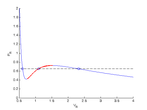
To find the areas, we need to know where the intersection of the vdW eqn with the horizontal line. This is the same as asking what are the roots of the vdW equation at that Pr. We need all three intersections so we can integrate from the first root to the middle root, and then the middle root to the third root. We take advantage of the polynomial nature of the vdW equation, which allows us to use the roots command to get all the roots at once. The polynomial is $V_R^3 - \frac{1}{3}(1+8 T_R/P_R) + 3/P_R - 1/P_R = 0$. We use the coefficients t0 get the rooys like this.
vdWp = [1 -1/3*(1+8*Tr/y) 3/y -1/y];
v = sort(roots(vdWp))
v =

    0.6029
    1.0974
    2.3253

plot the roots

we want to make sure the roots are really the intersections with the line.

plot(v(1),y,'bo',v(2),y,'bo',v(3),y,'bo')

compute areas

for A1, we need the area under the line minus the area under the vdW curve. That is the area between the curves. For A2, we want the area under the vdW curve minus the area under the line. The area under the line between root 2 and root 1 is just the width (root2 - root1)*y

A1 = (v(2)-v(1))*y - quad(Prfh,v(1),v(2))
A2 = quad(Prfh,v(2),v(3)) - (v(3)-v(2))*y
% these areas are pretty close, and we could iterate to get them very
% close. or, we can use a solver to do this. To do that, we need to define
% a function that is equal to zero when the two areas are equal. See the
% equalArea function below.

Pr_equal_area = fzero(@equalArea, 0.65)
A1 =

    0.0632


A2 =

    0.0580


Pr_equal_area =

    0.6470

confirm the two areas are equal

y = Pr_equal_area;
equalArea(y) % this should be close to zero
ans =

  1.1102e-016

and we can compute the areas too

vdWp = [1 -1/3*(1+8*Tr/y) 3/y -1/y]
v = sort(roots(vdWp))
A1 = (v(2)-v(1))*y - quad(Prfh,v(1),v(2))
A2 = quad(Prfh,v(2),v(3)) - (v(3)-v(2))*y
% these areas are very close to each other.
vdWp =

    1.0000   -4.0428    4.6368   -1.5456


v =

    0.6034
    1.0905
    2.3488


A1 =

    0.0618


A2 =

    0.0618

plot the areas that are equal

we want to show the areas that are equal by shading them.

xx = [v(1) Vr(Vr >= v(1) & Vr <= v(2)) v(2)];
yy = [Prfh(v(1)) Pr(Vr >= v(1) & Vr <= v(2)) Prfh(v(2))];
lightgray = [0.9 0.9 0.9];
fill(xx,yy,lightgray)

xx = [v(2) Vr(Vr >= v(2) & Vr <= v(3)) v(3)];
yy = [Prfh(v(2)) Pr(Vr >= v(2) & Vr <= v(3)) Prfh(v(3))];
fill(xx,yy,lightgray)
% and finally lets add text labels to the figure for what the areas are.
text(v(1),1,sprintf('A1 = %f',A1))
text(v(3),1,sprintf('A2 = %f',A2))

Finally, plot the isotherm

we want to replace the unstable region with the flat line that defines the equal areas. The roots are stored in the variable $v$. We use logical indexing to select the parts of the data that we want.
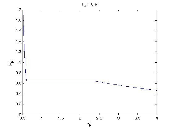
figure
Vrf = [Vr(Vr <= v(1)) v(1)       v(3)       Vr(Vr>= v(3))];
Prf = [Pr(Vr <= v(1)) Prfh(v(1)) Prfh(v(3)) Pr(Vr>= v(3))];
plot(Vrf,Prf)
ylim([0 2])
xlabel('V_R')
ylabel('P_R')
title('T_R = 0.9')

The flat line in this isotherm corresponds to a vapor-liquid equilibrium. This is the result for $T_R = 0.9$. You could also compute the isotherm for other $T_R$ values.

'done'
ans =

done

function Z = equalArea(y)
% compute A1 - A2 for Tr = 0.9.
Tr = 0.9;
vdWp = [1 -1/3*(1+8*Tr/y) 3/y -1/y];
v = sort(roots(vdWp));

Prfh = @(Vr) 8/3*Tr./(Vr - 1/3) - 3./(Vr.^2);
A1 = (v(2)-v(1))*y - quad(Prfh,v(1),v(2));
A2 = quad(Prfh,v(2),v(3)) - (v(3)-v(2))*y;

Z = A1 - A2;

% categories: Nonlinear algebra
% tags: thermodynamics
Read and Post Comments

Reading parameter database text files in Matlab

| categories: file io | View Comments

read_use_antoine

Contents

Reading parameter database text files in Matlab

John Kitchin

clear all; clc; close all

the datafile at http://terpconnect.umd.edu/~nsw/ench250/antoine.dat contains data that can be used to estimate the vapor pressure of about 700 pure compounds using the Antoine equation

The data file has the following contents:

 Antoine Coefficients
   log(P) = A-B/(T+C) where P is in mmHg and T is in Celsius
 Source of data: Yaws and Yang (Yaws, C.  L.  and Yang, H.  C.,
 "To estimate vapor pressure easily. antoine coefficients relate vapor pressure to temperature for almost 700 major organic compounds", Hydrocarbon Processing, 68(10), p65-68, 1989.
 ID  formula  compound name                  A       B       C     Tmin Tmax ??    ?
 -----------------------------------------------------------------------------------
   1 CCL4     carbon-tetrachloride        6.89410 1219.580 227.170  -20  101 Y2    0
   2 CCL3F    trichlorofluoromethane      6.88430 1043.010 236.860  -33   27 Y2    0

To use this data, you find the line that has the compound you want, and read off the data. You could do that manually for each component you want but that is tedious, and error prone. Today we will see how to retrieve the file, then read the data into Matlab to create a database we can use to store and retrieve the data.

We will use the data to find the temperature at which the vapor pressure of acetone is 400 mmHg.

get a local copy of the file

urlwrite('http://terpconnect.umd.edu/~nsw/ench250/antoine.dat','antoine_data.dat');

Reading in the data

We use the textscan command to skip the first 7 header lines, and then to parse each line according to the format string. After the header, each line has the format of:

 integer string string float float float float float string string

which we represent by '%d%s%s%f%f%f%f%f%s%s' as a format string. Note we are basically ignoring the contents of the last two columns, and just reading them in as strings. The output of the textread command will be a vector of values for each numerical column, and a cell array for string data.

now open it, and read it

the output of the textscan command is a cell array of all the data read in.

fid = fopen('antoine_data.dat');
C = textscan(fid,'%d%s%s%f%f%f%f%f%s%s','headerlines',7);
fclose(fid);

convert the cell array output of textscan into variables

This makes it easier to read the code where we assign the database. Each of these varialbes is a column vector containing the data for that column in our text file.

[id formula compound A B C Tmin Tmax i j] = C{:};

the database

the Map object will let us refer to an entry as database('acetone')

database = containers.Map();

storing the data

for i=1:length(id)
    % we store the data as a cell for each compound
    database(compound{i}) = {A(i) B(i) C(i) Tmin(i) Tmax(i)};
end
% That's it! Now, we can use the database to retrieve specific entries.

Now use the database to plot the vapor pressure of acetone

get the parameters for acetone

compound = database('acetone')
% for readability let's pull out each data property into variable names
[A B C Tmin Tmax] = compound{:}
compound = 

    [7.2316]    [1.2770e+003]    [237.2300]    [-32]    [77]


A =

    7.2316


B =

  1.2770e+003


C =

  237.2300


Tmin =

   -32


Tmax =

    77

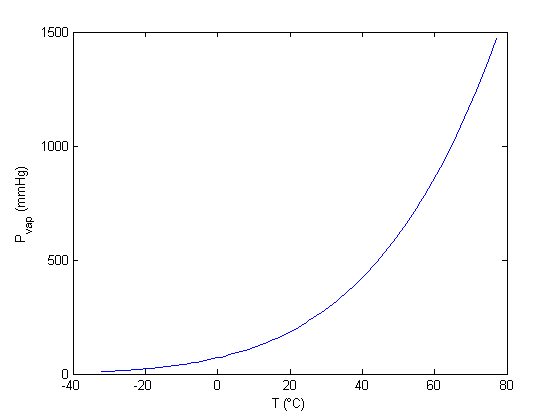
plot vapor pressure of acetone over the allowable temperature range.

T = linspace(Tmin, Tmax);
P = 10.^(A - B./(T+C));
plot(T,P)
xlabel('T (\circC)')
ylabel('P_{vap} (mmHg)')

Find T at which Pvap = 400 mmHg

from our graph we might guess T ~ 40 degC

Tguess = 40;
f = @(T) 400 - 10.^(A - B./(T+C));
T400 = fzero(f,Tguess)

sprintf('The vapor pressure is 400 mmHg at T = %1.1f degC',T400)
T400 =

   38.6138


ans =

The vapor pressure is 400 mmHg at T = 38.6 degC

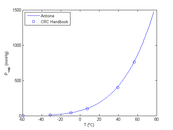
This result is close to the value reported here (39.5 degC), from the CRC Handbook. The difference is probably that the value reported in the CRC is an actual experimental number.

Plot CRC data

We only include the data for the range where the Antoine fit is valid.

T  = [-59.4 	-31.1 	-9.4 	7.7 	39.5 	56.5];
P = [	1 	10 	40 	100 	400 	760];

hold all
plot(T,P,'bo')
legend('Antoine','CRC Handbook','location','northwest')
% There is pretty good agreement between the Antoine equation and the data.

save the database for later use.

we can load this file into Matlab at a later time instead of reading in the text file again.

save  antoine_database.mat database

% categories: File IO
% tags: thermodynamics
Read and Post Comments

Constrained minimization to find equilibrium compositions

| categories: optimization | View Comments

Constrained minimization to find equilibrium compositions

Constrained minimization to find equilibrium compositions

adapated from Chemical Reactor analysis and design fundamentals, Rawlings and Ekerdt, appendix A.2.3.

Contents

The equilibrium composition of a reaction is the one that minimizes the total Gibbs free energy. The Gibbs free energy of a reacting ideal gas mixture depends on the mole fractions of each species, which are determined by the initial mole fractions of each species, the extent of reactions that convert each species, and the equilibrium constants.

Reaction 1: $I + B \rightleftharpoons P1$

Reaction 2: $I + B \rightleftharpoons P2$

The equilibrium constants for these reactions are known, and we seek to find the equilibrium reaction extents so we can determine equilibrium compositions.

function main
clc, close all, clear all

constraints

we have the following constraints, written in standard less than or equal to form:

$-\epsilon_1 \le 0$

$-\epsilon_2 \le 0$

$\epsilon_1 + \epsilon_2 \le 0.5$

We express this in matrix form as Ax=b where $A = \left[ \begin{array}{cc} -1 & 0 \\ 0 & -1 \\ 1 & 1 \end{array} \right]$ and $b = \left[ \begin{array}{c} 0 \\ 0 \\ 0.5\end{array} \right]$

A = [[-1 0];[0 -1];[1 1]];
b = [0;0;0.5];

% this is our initial guess
X0 = [0.1 0.1];

This does not work!

X = fmincon(@gibbs,X0,A,b)
Warning: Trust-region-reflective algorithm does not solve this type of
problem, using active-set algorithm. You could also try the interior-point or
sqp algorithms: set the Algorithm option to 'interior-point' or 'sqp' and
rerun. For more help, see Choosing the Algorithm in the documentation. 

Solver stopped prematurely.

fmincon stopped because it exceeded the function evaluation limit,
options.MaxFunEvals = 200 (the default value).


X =

      NaN +    NaNi      NaN +    NaNi

the error message suggests we try another solver. Here is how you do that.

options = optimset('Algorithm','interior-point');
X = fmincon(@gibbs,X0,A,b,[],[],[],[],[],options)
% note the options go at the end, so we have to put a lot of empty [] as
% placeholders for other inputs to fmincon.

% we can see what the gibbs energy is at our solution
gibbs(X)
Local minimum found that satisfies the constraints.

Optimization completed because the objective function is non-decreasing in 
feasible directions, to within the default value of the function tolerance,
and constraints were satisfied to within the default value of the constraint tolerance.


X =

    0.1334    0.3507


ans =

   -2.5594

getting the equilibrium compositions

these are simply mole balances to account for the consumption and production of each species

e1 = X(1);
e2 = X(2);

yI0 = 0.5; yB0 = 0.5; yP10 = 0; yP20 = 0; %initial mole fractions

d = 1 - e1 - e2;
yI = (yI0 - e1 - e2)/d;
yB = (yB0 - e1 - e2)/d;
yP1 = (yP10 + e1)/d;
yP2 = (yP20 + e2)/d;

sprintf('y_I = %1.3f y_B = %1.3f y_P1 = %1.3f y_P2 = %1.3f',yI,yB,yP1,yP2)
ans =

y_I = 0.031 y_B = 0.031 y_P1 = 0.258 y_P2 = 0.680

Verifying our solution

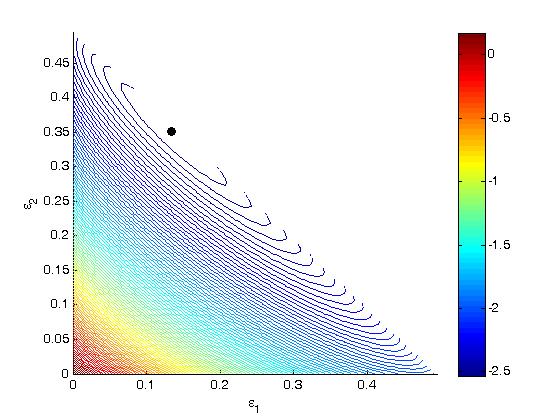
One way we can verify our solution is to plot the gibbs function and see where the minimum is, and whether there is more than one minimum. We start by making grids over the range of 0 to 0.5. Note we actually start slightly above zero because at zero there are some numerical imaginary elements of the gibbs function or it is numerically not defined since there are logs of zero there.

[E1, E2] = meshgrid(linspace(0.001,0.5),linspace(0.001,0.5));

% we have to remember that when e1 + e2 > 0.5, there is no solution to our
% gibbs functions, so we find the indices of the matrix where the sum is
% greater than 0.5, then we set those indices to 0 so no calculation gets
% done for them.
sumE = E1 + E2;
ind = sumE > 0.5;
E1(ind) = 0; E2(ind) = 0;

% we are going to use the arrayfun function to compute gibbs at each e1 and
% e2, but our gibbs function takes a vector input not two scalar inputs. So
% we create a function handle to call our gibbs function with two scalar
% values as a vector.
f = @(x,y) gibbs([x y]);

% finally, we compute gibbs at each reaction extent
G = arrayfun(f, E1, E2);

% and make a contour plot at the 100 levels
figure; hold all;
contour(E1,E2,G,100)
xlabel('\epsilon_1')
ylabel('\epsilon_2')

% let's add our solved solution to the contour plot
plot([X(1)],[X(2)],'ko','markerfacecolor','k')
colorbar
% you can see from this contour plot that there is only one minimum.
'done'
ans =

done

function retval = gibbs(X)
% we do not derive the form of this function here. See chapter 3.5 in the
% referenced text book.
e1 = X(1);
e2 = X(2);

K1 = 108; K2 = 284; P = 2.5;
yI0 = 0.5; yB0 = 0.5; yP10 = 0; yP20 = 0;

d = 1 - e1 - e2;
yI = (yI0 - e1 - e2)/d;
yB = (yB0 - e1 - e2)/d;
yP1 = (yP10 + e1)/d;
yP2 = (yP20 + e2)/d;

retval = -(e1*log(K1) + e2*log(K2)) + ...
    d*log(P) + yI*d*log(yI) + ...
    yB*d*log(yB) + yP1*d*log(yP1) + yP2*d*log(yP2);

% categories: Optimization
% tags: thermodynamics, reaction engineering
Read and Post Comments

polynomials in matlab

| categories: basic matlab | View Comments

polynomials

Contents

polynomials in matlab

polynomials can be represented as a vector of coefficients
4*x^3 + 3*x^2 -2*x + 10 = 0
can be represented as [4 3 -2 10]
ppar = [4 3 -2 10];

% we can evaluate the polynomial with the polyval command, e.g. to evaluate
% at x=3
polyval(ppar, 3)
ans =

   139

compare to

x=3;
4*x^3 + 3*x^2 -2*x + 10
% they are the same
ans =

   139

polynomial manipulations

matlab makes it easy to get the derivative and integral of a polynomial.

Consider:

$y = 2x^2 - 1$

ppar = [2 0 -1];

polynomial derivatives

$\frac{dy}{dx} = 4 x$

dpar = polyder(ppar)
% evaluate the derivative at x = 2
polyval(dpar,2)
dpar =

     4     0


ans =

     8

polynomial integrals

$\int y(x)dx = \frac{2}{3} x^3 - x + C$

We assume $C=0$.

ipar = polyint(ppar)
% note that the integration constant is assumed to be zero. If it is not
% zero, use POLYINT(P,K) where K is the constant of integration.
%
% Compute the integral of the polynomial from 2 to 4
polyval(ipar,4) - polyval(ipar,2)
% analytically:
2/3*(4^3 - 2^3) + (-4 - (-2))
ipar =

    0.6667         0   -1.0000         0


ans =

   35.3333


ans =

   35.3333

getting the roots of a polynomial

roots are the x-values that make the polynomial equal to zero.

roots(ppar)

% the analytical solutions are +- sqrt(1/2)

% note that imaginary roots exist, e.g. x^2 + 1 = 0 has two roots, +-i
ppar = [1 0 1]
roots(ppar)
ans =

    0.7071
   -0.7071


ppar =

     1     0     1


ans =

        0 + 1.0000i
        0 - 1.0000i

application in thermodynamics

we need to find the volume that solves the van der waal equation:

$$f(V) = V^3 - \frac{pnb + nRT}{p}V^2 + \frac{n^2a}{p}V - \frac{n^3ab}{p} = 0$$

where a and b are constants.

% numerical values of the constants
a = 3.49e4;
b = 1.45;
p = 679.7;
T = 683;
n = 1.136;
R = 10.73;

% The van der waal equation is a polynomial
%  V^3 - (p*n*b+n*R*T)/p*V^2 + n^2*a/p*V - n^3*a*b/p = 0

%use commas for clarity in separation of terms
ppar = [1, -(p*n*b+n*R*T)/p, n^2*a/p,  -n^3*a*b/p];
roots(ppar)

% note that only one root is real. In this case that means there is only
% one phase present.

% categories: Basic matlab
% tags: math, thermodynamics
ans =

   5.0943          
   4.4007 + 1.4350i
   4.4007 - 1.4350i

Read and Post Comments

« Previous Page