Constrained minimization to find equilibrium compositions

adapated from Chemical Reactor analysis and design fundamentals, Rawlings and Ekerdt, appendix A.2.3.

Contents

The equilibrium composition of a reaction is the one that minimizes the total Gibbs free energy. The Gibbs free energy of a reacting ideal gas mixture depends on the mole fractions of each species, which are determined by the initial mole fractions of each species, the extent of reactions that convert each species, and the equilibrium constants.

Reaction 1:

Reaction 2:

The equilibrium constants for these reactions are known, and we seek to find the equilibrium reaction extents so we can determine equilibrium compositions.

function main

clc, close all, clear all

constraints

we have the following constraints, written in standard less than or equal to form:

We express this in matrix form as Ax=b where and

A = [[-1 0];[0 -1];[1 1]];
b = [0;0;0.5];

% this is our initial guess
X0 = [0.1 0.1];

This does not work!

X = fmincon(@gibbs,X0,A,b)

Warning: Trust-region-reflective algorithm does not solve this type of
problem, using active-set algorithm. You could also try the interior-point or
sqp algorithms: set the Algorithm option to 'interior-point' or 'sqp' and
rerun. For more help, see Choosing the Algorithm in the documentation. 

Solver stopped prematurely.

fmincon stopped because it exceeded the function evaluation limit,
options.MaxFunEvals = 200 (the default value).


X =

      NaN +    NaNi      NaN +    NaNi

the error message suggests we try another solver. Here is how you do that.

options = optimset('Algorithm','interior-point');
X = fmincon(@gibbs,X0,A,b,[],[],[],[],[],options)
% note the options go at the end, so we have to put a lot of empty [] as
% placeholders for other inputs to fmincon.

% we can see what the gibbs energy is at our solution
gibbs(X)

Local minimum found that satisfies the constraints.

Optimization completed because the objective function is non-decreasing in 
feasible directions, to within the default value of the function tolerance,
and constraints were satisfied to within the default value of the constraint tolerance.




X =

    0.1334    0.3507


ans =

   -2.5594

getting the equilibrium compositions

these are simply mole balances to account for the consumption and production of each species

e1 = X(1);
e2 = X(2);

yI0 = 0.5; yB0 = 0.5; yP10 = 0; yP20 = 0; %initial mole fractions

d = 1 - e1 - e2;
yI = (yI0 - e1 - e2)/d;
yB = (yB0 - e1 - e2)/d;
yP1 = (yP10 + e1)/d;
yP2 = (yP20 + e2)/d;

sprintf('y_I = %1.3f y_B = %1.3f y_P1 = %1.3f y_P2 = %1.3f',yI,yB,yP1,yP2)

ans =

y_I = 0.031 y_B = 0.031 y_P1 = 0.258 y_P2 = 0.680

Verifying our solution

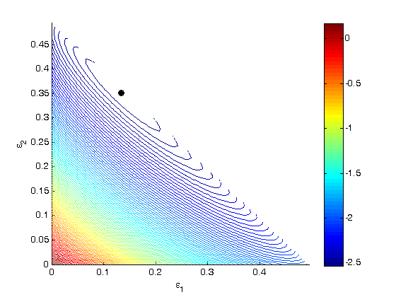
One way we can verify our solution is to plot the gibbs function and see where the minimum is, and whether there is more than one minimum. We start by making grids over the range of 0 to 0.5. Note we actually start slightly above zero because at zero there are some numerical imaginary elements of the gibbs function or it is numerically not defined since there are logs of zero there.

[E1, E2] = meshgrid(linspace(0.001,0.5),linspace(0.001,0.5));

% we have to remember that when e1 + e2 > 0.5, there is no solution to our
% gibbs functions, so we find the indices of the matrix where the sum is
% greater than 0.5, then we set those indices to 0 so no calculation gets
% done for them.
sumE = E1 + E2;
ind = sumE > 0.5;
E1(ind) = 0; E2(ind) = 0;

% we are going to use the arrayfun function to compute gibbs at each e1 and
% e2, but our gibbs function takes a vector input not two scalar inputs. So
% we create a function handle to call our gibbs function with two scalar
% values as a vector.
f = @(x,y) gibbs([x y]);

% finally, we compute gibbs at each reaction extent
G = arrayfun(f, E1, E2);

% and make a contour plot at the 100 levels
figure; hold all;
contour(E1,E2,G,100)
xlabel('\epsilon_1')
ylabel('\epsilon_2')

% let's add our solved solution to the contour plot
plot([X(1)],[X(2)],'ko','markerfacecolor','k')
colorbar
% you can see from this contour plot that there is only one minimum.

'done'

ans =

done

function retval = gibbs(X)
% we do not derive the form of this function here. See chapter 3.5 in the
% referenced text book.
e1 = X(1);
e2 = X(2);

K1 = 108; K2 = 284; P = 2.5;
yI0 = 0.5; yB0 = 0.5; yP10 = 0; yP20 = 0;

d = 1 - e1 - e2;
yI = (yI0 - e1 - e2)/d;
yB = (yB0 - e1 - e2)/d;
yP1 = (yP10 + e1)/d;
yP2 = (yP20 + e2)/d;

retval = -(e1*log(K1) + e2*log(K2)) + ...
    d*log(P) + yI*d*log(yI) + ...
    yB*d*log(yB) + yP1*d*log(yP1) + yP2*d*log(yP2);

% categories: Optimization
% tags: thermodynamics, reaction engineering

Published with MATLAB® 7.10