Reading parameter database text files in Matlab
September 10, 2011 at 06:31 PM | categories: file io | View Comments
Contents
- Reading parameter database text files in Matlab
- get a local copy of the file
- Reading in the data
- now open it, and read it
- convert the cell array output of textscan into variables
- the database
- storing the data
- Now use the database to plot the vapor pressure of acetone
- plot vapor pressure of acetone over the allowable temperature range.
- Find T at which Pvap = 400 mmHg
- Plot CRC data
- save the database for later use.
Reading parameter database text files in Matlab
John Kitchin
clear all; clc; close all
the datafile at http://terpconnect.umd.edu/~nsw/ench250/antoine.dat contains data that can be used to estimate the vapor pressure of about 700 pure compounds using the Antoine equation
The data file has the following contents:
 Antoine Coefficients
   log(P) = A-B/(T+C) where P is in mmHg and T is in Celsius
 Source of data: Yaws and Yang (Yaws, C.  L.  and Yang, H.  C.,
 "To estimate vapor pressure easily. antoine coefficients relate vapor pressure to temperature for almost 700 major organic compounds", Hydrocarbon Processing, 68(10), p65-68, 1989.
 ID  formula  compound name                  A       B       C     Tmin Tmax ??    ?
 -----------------------------------------------------------------------------------
   1 CCL4     carbon-tetrachloride        6.89410 1219.580 227.170  -20  101 Y2    0
   2 CCL3F    trichlorofluoromethane      6.88430 1043.010 236.860  -33   27 Y2    0
To use this data, you find the line that has the compound you want, and read off the data. You could do that manually for each component you want but that is tedious, and error prone. Today we will see how to retrieve the file, then read the data into Matlab to create a database we can use to store and retrieve the data.
We will use the data to find the temperature at which the vapor pressure of acetone is 400 mmHg.
get a local copy of the file
urlwrite('http://terpconnect.umd.edu/~nsw/ench250/antoine.dat','antoine_data.dat');
Reading in the data
We use the textscan command to skip the first 7 header lines, and then to parse each line according to the format string. After the header, each line has the format of:
integer string string float float float float float string string
which we represent by '%d%s%s%f%f%f%f%f%s%s' as a format string. Note we are basically ignoring the contents of the last two columns, and just reading them in as strings. The output of the textread command will be a vector of values for each numerical column, and a cell array for string data.
now open it, and read it
the output of the textscan command is a cell array of all the data read in.
fid = fopen('antoine_data.dat');
C = textscan(fid,'%d%s%s%f%f%f%f%f%s%s','headerlines',7);
fclose(fid);
convert the cell array output of textscan into variables
This makes it easier to read the code where we assign the database. Each of these varialbes is a column vector containing the data for that column in our text file.
[id formula compound A B C Tmin Tmax i j] = C{:};
the database
the Map object will let us refer to an entry as database('acetone')
database = containers.Map();
storing the data
for i=1:length(id)
    % we store the data as a cell for each compound
    database(compound{i}) = {A(i) B(i) C(i) Tmin(i) Tmax(i)};
end
% That's it! Now, we can use the database to retrieve specific entries.
Now use the database to plot the vapor pressure of acetone
get the parameters for acetone
compound = database('acetone')
% for readability let's pull out each data property into variable names
[A B C Tmin Tmax] = compound{:}
compound =

    [7.2316]    [1.2770e+003]    [237.2300]    [-32]    [77]


A =

    7.2316


B =

  1.2770e+003


C =

  237.2300


Tmin =

   -32


Tmax =

    77
plot vapor pressure of acetone over the allowable temperature range.
T = linspace(Tmin, Tmax);
P = 10.^(A - B./(T+C));
plot(T,P)
xlabel('T (\circC)')
ylabel('P_{vap} (mmHg)')
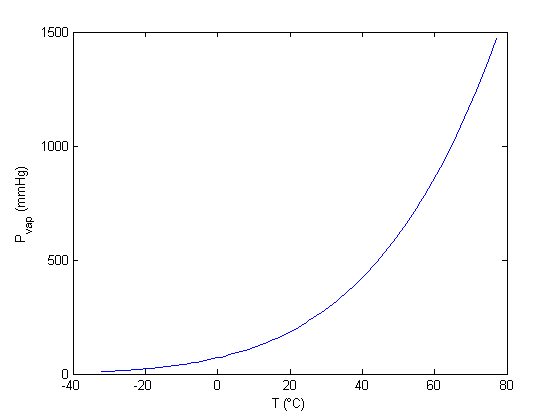
Find T at which Pvap = 400 mmHg
from our graph we might guess T ~ 40 degC
Tguess = 40;
f = @(T) 400 - 10.^(A - B./(T+C));
T400 = fzero(f,Tguess)

sprintf('The vapor pressure is 400 mmHg at T = %1.1f degC',T400)
T400 =

   38.6138


ans =

The vapor pressure is 400 mmHg at T = 38.6 degC
This result is close to the value reported here (39.5 degC), from the CRC Handbook. The difference is probably that the value reported in the CRC is an actual experimental number.
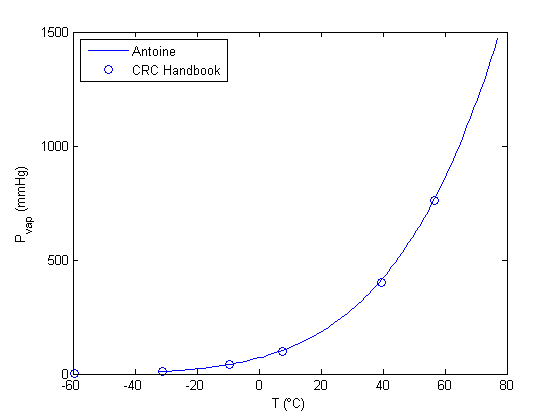
Plot CRC data
We only include the data for the range where the Antoine fit is valid.
T  = [-59.4 	-31.1 	-9.4 	7.7 	39.5 	56.5];
P = [	1 	10 	40 	100 	400 	760];

hold all
plot(T,P,'bo')
legend('Antoine','CRC Handbook','location','northwest')
% There is pretty good agreement between the Antoine equation and the data.
save the database for later use.
we can load this file into Matlab at a later time instead of reading in the text file again.
save  antoine_database.mat database

% categories: File IO
% tags: thermodynamics
 . We can read each cell. We can also write a value to B1, and then read B2 to get the value squared. finally, we will create a function that uses Excel to perform the calculation of squaring a number, and use fsolve to minimize the function.
 . We try guesses above and below each one.