Introduction to statistical data analysis

| categories: data analysis | View Comments

statistics

Contents

Introduction to statistical data analysis

clear all
clc

Problem statement.

Given several measurements of a single quantity, determine the average value of the measurements, the standard deviation of the measurements and the 95% confidence interval for the average.

the data

y = [8.1 8.0 8.1];

the average and standard deviation

ybar = mean(y)
s = std(y)
ybar =

    8.0667


s =

    0.0577

the confidence interval

This is a recipe for computing the confidence interval. The strategy is:
  1. compute the average
  2. Compute the standard deviation of your data
  3. Define the confidence interval, e.g. 95% = 0.95
  4. compute the student-t multiplier. This is a function of the confidence interval you specify, and the number of data points you have minus 1. You subtract 1 because one degree of freedom is lost from calculating the average.

The confidence interval is defined as ybar +- T_multiplier*std/sqrt(n).

the tinv command provides the T_multiplier

ci = 0.95;
alpha = 1 - ci;

n = length(y); %number of elements in the data vector
T_multiplier = tinv(1-alpha/2, n-1)
% the multiplier is large here because there is so little data. That means
% we do not have a lot of confidence on the true average or standard
% deviation
ci95 = T_multiplier*s/sqrt(n)

% confidence interval
sprintf('The confidence interval is %1.1f +- %1.1f',ybar,ci95)
[ybar - ci95, ybar + ci95]

% we can say with 95% confidence that the true mean lies between these two
% values.

% categories: Data analysis
T_multiplier =

    4.3027


ci95 =

    0.1434


ans =

The confidence interval is 8.1 +- 0.1


ans =

    7.9232    8.2101
Read and Post Comments

plotting two datasets with very different scales

| categories: plotting | View Comments

subplots

Contents

plotting two datasets with very different scales

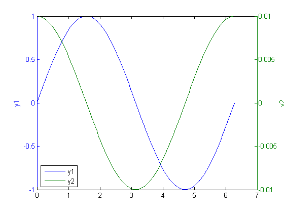
sometimes you will have two datasets you want to plot together, but the scales will be so different it is hard to seem them both in the same plot. Here we examine a few strategies to plotting this kind of data.

x = linspace(0,2*pi);
y1 = sin(x);
y2 = 0.01*cos(x);

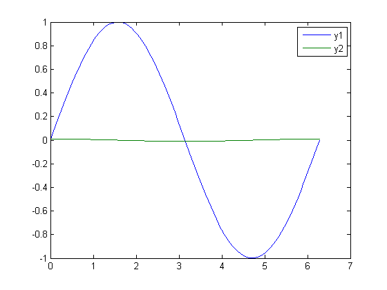
plot(x,y1,x,y2)
legend('y1','y2')
% in this plot y2 looks almost flat!

make two plots!

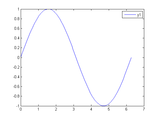
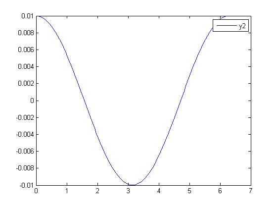
this certainly solves the problem, but you have two full size plots, which can take up a lot of space in a presentation and report. Often your goal in plotting both data sets is to compare them, and it is easiest to compare plots when they are perfectly lined up. Doing that manually can be tedious.

plot(x,y1); legend('y1')
plot(x,y2); legend('y2')

Scaling the results

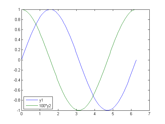
sometimes you can scale one dataset so it has a similar magnitude as the other data set. Here we could multiply y2 by 100, and then it will be similar in size to y1. Of course, you need to indicate that y2 has been scaled in the graph somehow. Here we use the legend.

plot(x,y1,x,100*y2)
legend('y1','100*y2','location','southwest')

double-y axis plot

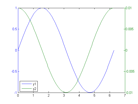
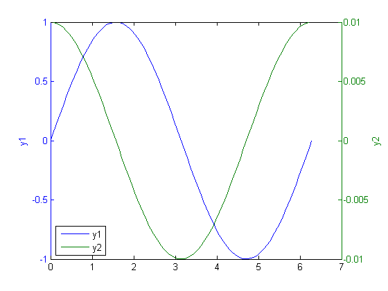
using two separate y-axes can solve your scaling problem. Note that each y-axis is color coded to the data. It can be difficult to read these graphs when printed in black and white

plotyy(x,y1,x,y2)
legend('y1','y2','location','southwest')

Setting the ylabels on these graphs is trickier than usual.

[AX,H1,H2] = plotyy(x,y1,x,y2)
legend('y1','y2','location','southwest')
set(get(AX(1),'Ylabel'),'String','y1')
set(get(AX(2),'Ylabel'),'String','y2')
AX =

  409.0186  411.0195


H1 =

  410.0281


H2 =

  412.0215

note that y2 is cut off just a little. We need to modify the axes position to decrease the width.

p = get(AX(1),'Position') % [x y width height]
% The width is too large, so let's decrease it a little
p(3)=0.75;

set(AX(1),'Position',p) % it doesn't seem to matter which axes we modify
p =

    0.1300    0.1100    0.7750    0.8150

subplots

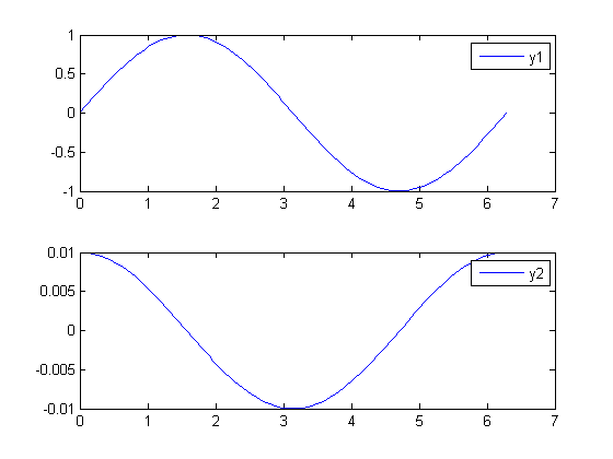
an alternative approach to double y axes is to use subplots. The subplot command has a syntax of subplot(m,n,p) which selects the p-th plot in an m by n array of plots. Then you use a regular plot command to put your figure there. Here we stack two plots in a 2 (row) by 1 (column).

subplot(2,1,1)
plot(x,y1); legend('y1')

subplot(2,1,2)
plot(x,y2); legend('y2')
'done'
% categories: plotting
ans =

done

Read and Post Comments

Indexing vectors and arrays in Matlab

| categories: basic matlab | View Comments

Indexing vectors and arrays in Matlab

Indexing vectors and arrays in Matlab

There are times where you have a lot of data in a vector or array and you want to extract a portion of the data for some analysis. For example, maybe you want to plot column 1 vs column 2, or you want the integral of data between x = 4 and x = 6, but your vector covers 0 < x < 10. Indexing is the way to do these things.

A key point to remember is that in Matlab array/vector indices start at 1.

Contents

we use the parentheses operator to index. It is possible to get a single element, a range of elements, or all the elements.

x = linspace(0,pi,10)
x =

  Columns 1 through 7

         0    0.3491    0.6981    1.0472    1.3963    1.7453    2.0944

  Columns 8 through 10

    2.4435    2.7925    3.1416

x(1)   % element 1
ans =

     0

x(3)   % element 3
ans =

    0.6981

x(1:3) % elements 1-3
ans =

         0    0.3491    0.6981

x(end) % the last element
ans =

    3.1416

the syntax a:n:b gets the elements starting at index a, skipping n elements up to the index b

x(1:3:end) % every third element
ans =

         0    1.0472    2.0944    3.1416

x(:) % getting all the elements. :note:`you get a column vector.`
ans =

         0
    0.3491
    0.6981
    1.0472
    1.3963
    1.7453
    2.0944
    2.4435
    2.7925
    3.1416

finding part of vector

suppose we want the part of the vector where x > 2. We could do that by inspection, but there is a better way. We can create a mask of boolean (0 or 1) values that specify whether x > 2 or not, and then use the mask

ind = x > 2
x(ind) % use indexing to get the part of x where x > 2
ind =

     0     0     0     0     0     0     1     1     1     1


ans =

    2.0944    2.4435    2.7925    3.1416

we can use the mask on other vectors too, to get the y-values where x > 2, for example, and then to integrate that subsection of data (or some other analysis).

y = sin(x)
y(ind)
trapz(y(ind),x(ind))
y =

  Columns 1 through 7

         0    0.3420    0.6428    0.8660    0.9848    0.9848    0.8660

  Columns 8 through 10

    0.6428    0.3420    0.0000


ans =

    0.8660    0.6428    0.3420    0.0000


ans =

   -2.3087

2D array indexing

in a 2D array, you index with (row,column)

a = [[1 2 3];[4 5 6]; [7 8 9]]
a =

     1     2     3
     4     5     6
     7     8     9

a(1,1) % upper left element
a(end,end) % lower right element
ans =

     1


ans =

     9

getting a row

to get a row, we specify the row number we want, and we need a syntax to specify every column index in that row. The syntax is to use a colon

a(1,:) % first row
ans =

     1     2     3

getting a column

a(:,1) % first column
ans =

     1
     4
     7

a(:) % all the elements of the a array as a column vector
ans =

     1
     4
     7
     2
     5
     8
     3
     6
     9

using indexing to assign values to rows and columns

b = zeros(size(a))
b =

     0     0     0
     0     0     0
     0     0     0

b(:,1) = [1 2 3] % define column 1
b =

     1     0     0
     2     0     0
     3     0     0

b(2,:) = [4 5 6] % define row 2
b =

     1     0     0
     4     5     6
     3     0     0

b(3,3) = 9 % define element (3,3)
b =

     1     0     0
     4     5     6
     3     0     9

b(9) = 12  % this redefines element (3,3)
b =

     1     0     0
     4     5     6
     3     0    12

3D arrays

the 3d array is like book of 2D matrices. Each page has a 2D matrix on it. think about the indexing like this: (row, column, page)

M = randn(3,3,3) % a 3x3x3 array
M(:,:,1) =

    1.7119   -0.8396    0.9610
   -0.1941    1.3546    0.1240
   -2.1384   -1.0722    1.4367


M(:,:,2) =

   -1.9609    2.9080   -1.0582
   -0.1977    0.8252   -0.4686
   -1.2078    1.3790   -0.2725


M(:,:,3) =

    1.0984   -2.0518   -1.5771
   -0.2779   -0.3538    0.5080
    0.7015   -0.8236    0.2820

M(:,:,1) % 2D array on page 1
ans =

    1.7119   -0.8396    0.9610
   -0.1941    1.3546    0.1240
   -2.1384   -1.0722    1.4367

M(:,1,1) % column 1 of array on page 1
ans =

    1.7119
   -0.1941
   -2.1384

M(2,:,2) % row 2 of array on page 2
ans =

   -0.1977    0.8252   -0.4686

Wrapup

The most common place to use indexing is probably when a function returns an array with the independent variable in column 1 and solution in column 2, and you want to plot the solution. Second is when you want to analyze one part of the solution. There are also applications in numerical methods, for example in assigning values to the elements of a matrix or vector.

% categories: basic matlab

% post_id = 916; %delete this line to force new post;
Read and Post Comments

transient heat conduction - partial differential equations

| categories: pdes | View Comments

transient heat conduction - partial differential equations

transient heat conduction - partial differential equations

adapated from http://msemac.redwoods.edu/~darnold/math55/DEproj/sp02/AbeRichards/slideshowdefinal.pdf

Contents

In Post 860 we solved a steady state BVP modeling heat conduction. Today we examine the transient behavior of a rod at constant T put between two heat reservoirs at different temperatures, again T1 = 100, and T2 = 200. The rod will start at 150. Over time, we should expect a solution that approaches the steady state solution: a linear temperature profile from one side of the rod to the other.

$\frac{\partial u}{\partial t} = k \frac{\partial^2 u}{\partial x^2}$

at $t=0$, in this example we have $u_0(x) = 150$ as an initial condition. with boundary conditions $u(0,t)=100$ and $u(L,t)=200$.

Matlab provides the pdepe command which can solve some PDEs. The syntax for the command is

 sol = pdepe(m,@pdex,@pdexic,@pdexbc,x,t)

where m is an integer that specifies the problem symmetry. The three function handles define the equations, initial conditions and boundary conditions. x and t are the grids to solve the PDE on.

function pdexfunc
close all; clc; clear all;

setup the problem

m=0; % specifies 1-D symmetry
x = linspace(0,1); % equally-spaced points along the length of the rod
t = linspace(0,5); % this creates time points

sol = pdepe(m,@pdex,@pdexic,@pdexbc,x,t);

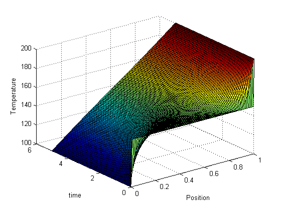
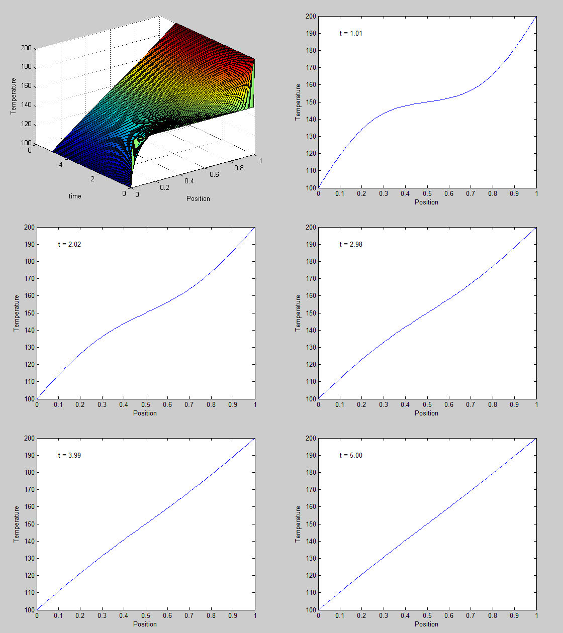
plot the solution as a 3D surface

x is the position along the rod, t is the time sol is the temperature at (x,t)

surf(x,t,sol)
xlabel('Position')
ylabel('time')
zlabel('Temperature')

in the surface plot above you can see the approach from the initial conditions to the steady state solution.

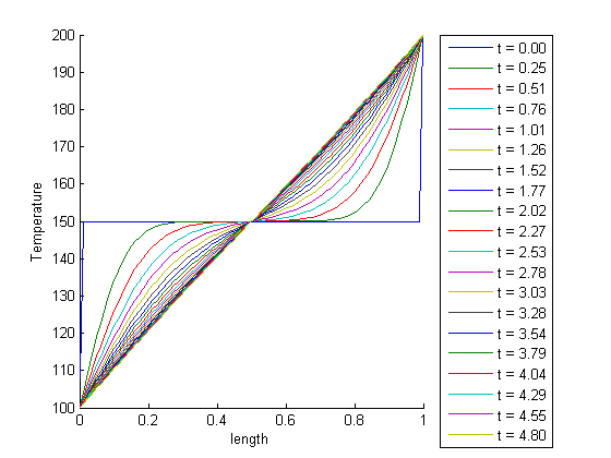
we can also plot the solutions in 2D, at different times. Our time vector has about 100 elements, so in this loop we plot every 5th time. We set a DisplayName in each plot so we can use them in the legend later.

figure
hold all % the use of all makes the colors cycle with each plot
for i=1:5:numel(t)
    plot(x,sol(i,:),'DisplayName',sprintf('t = %1.2f',t(i)))
end
xlabel('length')
ylabel('Temperature')

% we use -DynamicLegend to pick up the display names we set above.
legend('-DynamicLegend','location','bestoutside');
% this is not an easy way to see the solution.

animating the solution

we can create an animated gif to show how the solution evolves over time.

filename = 'animated-solution.gif'; % file to store image in
for i=1:numel(t)
    plot(x,sol(i,:));
    xlabel('Position')
    ylabel('Temperature')
    text(0.1,190,sprintf('t = %1.2f',t(i))); % add text annotation of time step
    frame = getframe(1);
    im = frame2im(frame); %convert frame to an image
    [imind,cm] = rgb2ind(im,256);

    % now we write out the image to the animated gif.
    if i == 1;
        imwrite(imind,cm,filename,'gif', 'Loopcount',inf);
    else
        imwrite(imind,cm,filename,'gif','WriteMode','append');
    end
end
close all; % makes sure the plot from the loop above doesn't get published

here is the animation!

It is slightly more clear that the temperature profile evolves from a flat curve, to a linear temperature ramp between the two end points.

'done'
ans =

done

function [c,f,s] = pdex(x,t,u,DuDx)

For pdepe to understand the equations, they need to be in the form of

$c(x,t,u,\frac{\partial u}{\partial x}) \frac{\partial u}{\partial t} = x^{-m} \frac{\partial}{\partial x}(x^m f(x,t,u,\frac{\partial u}{\partial x})) + s(x,t,u,\frac{\partial u}{\partial x})$

where c is a diagonal matrix, f is called a flux term, and s is the source term. Our equations are:

$$1(\frac{\partial u}{\partial t}) = \frac{\partial }{\partial x}(k \frac{\partial u}{\partial x})$$

from which you can see that $c=1$, $f = k\frac{\partial u}{\partial x}$, and $s=0$

c = 1;
f = 0.02*DuDx;
s = 0;
function u0 = pdexic(x)
% this defines u(t=0) for all of x. The problem specifies a constant T for
% all of x.
u0 = 150;

function [p1,q1,pr,qr] = pdexbc(x1,u1,xr,ur,t)
% this defines the boundary conditions. The general form of the boundary
% conditions are $p(x,t,u) + q(x,t)f(x,t,u,\frac{\partial u}{\partial x})$
% We have to define the boundary conditions on the left, and right.
p1 = u1-100; % at left
q1 = 0; % at left
pr= ur-200;  % at right
qr = 0; % at right


% categories: PDEs
% tags: heat transfer
Read and Post Comments

Constrained minimization to find equilibrium compositions

| categories: optimization | View Comments

Constrained minimization to find equilibrium compositions

Constrained minimization to find equilibrium compositions

adapated from Chemical Reactor analysis and design fundamentals, Rawlings and Ekerdt, appendix A.2.3.

Contents

The equilibrium composition of a reaction is the one that minimizes the total Gibbs free energy. The Gibbs free energy of a reacting ideal gas mixture depends on the mole fractions of each species, which are determined by the initial mole fractions of each species, the extent of reactions that convert each species, and the equilibrium constants.

Reaction 1: $I + B \rightleftharpoons P1$

Reaction 2: $I + B \rightleftharpoons P2$

The equilibrium constants for these reactions are known, and we seek to find the equilibrium reaction extents so we can determine equilibrium compositions.

function main
clc, close all, clear all

constraints

we have the following constraints, written in standard less than or equal to form:

$-\epsilon_1 \le 0$

$-\epsilon_2 \le 0$

$\epsilon_1 + \epsilon_2 \le 0.5$

We express this in matrix form as Ax=b where $A = \left[ \begin{array}{cc} -1 & 0 \\ 0 & -1 \\ 1 & 1 \end{array} \right]$ and $b = \left[ \begin{array}{c} 0 \\ 0 \\ 0.5\end{array} \right]$

A = [[-1 0];[0 -1];[1 1]];
b = [0;0;0.5];

% this is our initial guess
X0 = [0.1 0.1];

This does not work!

X = fmincon(@gibbs,X0,A,b)
Warning: Trust-region-reflective algorithm does not solve this type of
problem, using active-set algorithm. You could also try the interior-point or
sqp algorithms: set the Algorithm option to 'interior-point' or 'sqp' and
rerun. For more help, see Choosing the Algorithm in the documentation. 

Solver stopped prematurely.

fmincon stopped because it exceeded the function evaluation limit,
options.MaxFunEvals = 200 (the default value).


X =

      NaN +    NaNi      NaN +    NaNi

the error message suggests we try another solver. Here is how you do that.

options = optimset('Algorithm','interior-point');
X = fmincon(@gibbs,X0,A,b,[],[],[],[],[],options)
% note the options go at the end, so we have to put a lot of empty [] as
% placeholders for other inputs to fmincon.

% we can see what the gibbs energy is at our solution
gibbs(X)
Local minimum found that satisfies the constraints.

Optimization completed because the objective function is non-decreasing in 
feasible directions, to within the default value of the function tolerance,
and constraints were satisfied to within the default value of the constraint tolerance.


X =

    0.1334    0.3507


ans =

   -2.5594

getting the equilibrium compositions

these are simply mole balances to account for the consumption and production of each species

e1 = X(1);
e2 = X(2);

yI0 = 0.5; yB0 = 0.5; yP10 = 0; yP20 = 0; %initial mole fractions

d = 1 - e1 - e2;
yI = (yI0 - e1 - e2)/d;
yB = (yB0 - e1 - e2)/d;
yP1 = (yP10 + e1)/d;
yP2 = (yP20 + e2)/d;

sprintf('y_I = %1.3f y_B = %1.3f y_P1 = %1.3f y_P2 = %1.3f',yI,yB,yP1,yP2)
ans =

y_I = 0.031 y_B = 0.031 y_P1 = 0.258 y_P2 = 0.680

Verifying our solution

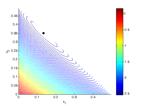
One way we can verify our solution is to plot the gibbs function and see where the minimum is, and whether there is more than one minimum. We start by making grids over the range of 0 to 0.5. Note we actually start slightly above zero because at zero there are some numerical imaginary elements of the gibbs function or it is numerically not defined since there are logs of zero there.

[E1, E2] = meshgrid(linspace(0.001,0.5),linspace(0.001,0.5));

% we have to remember that when e1 + e2 > 0.5, there is no solution to our
% gibbs functions, so we find the indices of the matrix where the sum is
% greater than 0.5, then we set those indices to 0 so no calculation gets
% done for them.
sumE = E1 + E2;
ind = sumE > 0.5;
E1(ind) = 0; E2(ind) = 0;

% we are going to use the arrayfun function to compute gibbs at each e1 and
% e2, but our gibbs function takes a vector input not two scalar inputs. So
% we create a function handle to call our gibbs function with two scalar
% values as a vector.
f = @(x,y) gibbs([x y]);

% finally, we compute gibbs at each reaction extent
G = arrayfun(f, E1, E2);

% and make a contour plot at the 100 levels
figure; hold all;
contour(E1,E2,G,100)
xlabel('\epsilon_1')
ylabel('\epsilon_2')

% let's add our solved solution to the contour plot
plot([X(1)],[X(2)],'ko','markerfacecolor','k')
colorbar
% you can see from this contour plot that there is only one minimum.
'done'
ans =

done

function retval = gibbs(X)
% we do not derive the form of this function here. See chapter 3.5 in the
% referenced text book.
e1 = X(1);
e2 = X(2);

K1 = 108; K2 = 284; P = 2.5;
yI0 = 0.5; yB0 = 0.5; yP10 = 0; yP20 = 0;

d = 1 - e1 - e2;
yI = (yI0 - e1 - e2)/d;
yB = (yB0 - e1 - e2)/d;
yP1 = (yP10 + e1)/d;
yP2 = (yP20 + e2)/d;

retval = -(e1*log(K1) + e2*log(K2)) + ...
    d*log(P) + yI*d*log(yI) + ...
    yB*d*log(yB) + yP1*d*log(yP1) + yP2*d*log(yP2);

% categories: Optimization
% tags: thermodynamics, reaction engineering
Read and Post Comments

« Previous Page -- Next Page »