Matlab in Chemical Engineering at CMU

Contents

plotting two datasets with very different scales

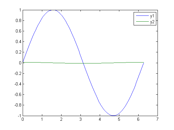
sometimes you will have two datasets you want to plot together, but the scales will be so different it is hard to seem them both in the same plot. Here we examine a few strategies to plotting this kind of data.

x = linspace(0,2*pi);
y1 = sin(x);
y2 = 0.01*cos(x);

plot(x,y1,x,y2)
legend('y1','y2')
% in this plot y2 looks almost flat!

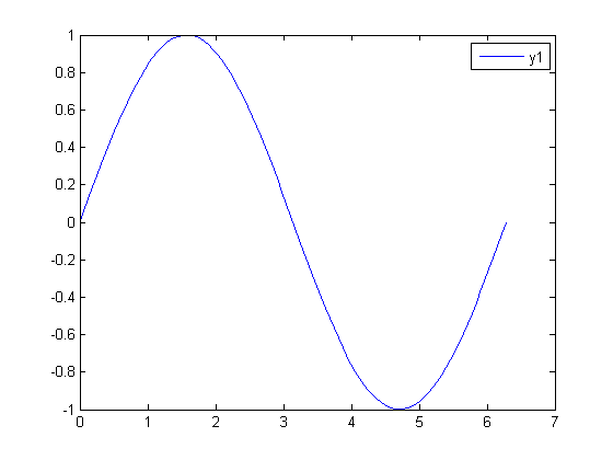
make two plots!

this certainly solves the problem, but you have two full size plots, which can take up a lot of space in a presentation and report. Often your goal in plotting both data sets is to compare them, and it is easiest to compare plots when they are perfectly lined up. Doing that manually can be tedious.

plot(x,y1); legend('y1')

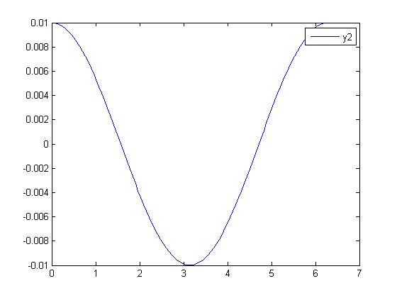
plot(x,y2); legend('y2')

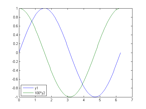
Scaling the results

sometimes you can scale one dataset so it has a similar magnitude as the other data set. Here we could multiply y2 by 100, and then it will be similar in size to y1. Of course, you need to indicate that y2 has been scaled in the graph somehow. Here we use the legend.

plot(x,y1,x,100*y2)
legend('y1','100*y2','location','southwest')

double-y axis plot

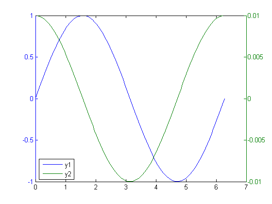
using two separate y-axes can solve your scaling problem. Note that each y-axis is color coded to the data. It can be difficult to read these graphs when printed in black and white

plotyy(x,y1,x,y2)
legend('y1','y2','location','southwest')

Setting the ylabels on these graphs is trickier than usual.

[AX,H1,H2] = plotyy(x,y1,x,y2)
legend('y1','y2','location','southwest')
set(get(AX(1),'Ylabel'),'String','y1')
set(get(AX(2),'Ylabel'),'String','y2')

AX =

  409.0186  411.0195


H1 =

  410.0281


H2 =

  412.0215

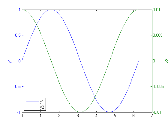
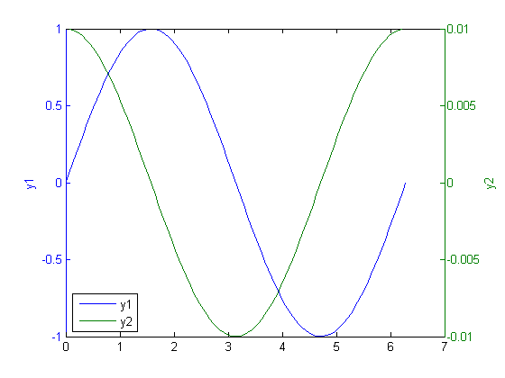
note that y2 is cut off just a little. We need to modify the axes position to decrease the width.

p = get(AX(1),'Position') % [x y width height]
% The width is too large, so let's decrease it a little
p(3)=0.75;

set(AX(1),'Position',p) % it doesn't seem to matter which axes we modify

p =

    0.1300    0.1100    0.7750    0.8150

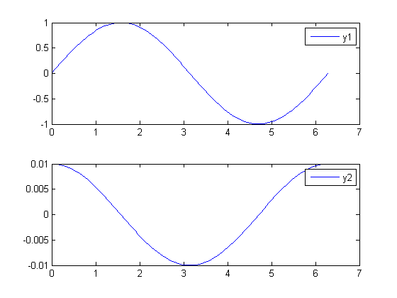
subplots

an alternative approach to double y axes is to use subplots. The subplot command has a syntax of subplot(m,n,p) which selects the p-th plot in an m by n array of plots. Then you use a regular plot command to put your figure there. Here we stack two plots in a 2 (row) by 1 (column).

subplot(2,1,1)
plot(x,y1); legend('y1')

subplot(2,1,2)
plot(x,y2); legend('y2')

'done'
% categories: plotting

ans =

done

Published with MATLAB® 7.10