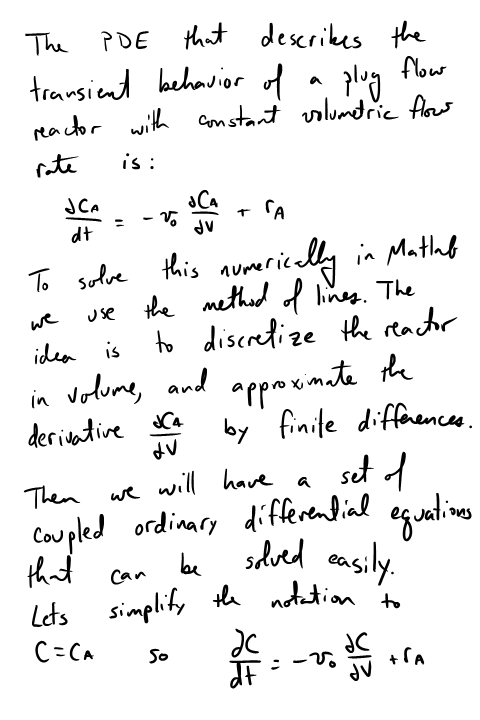
Modeling a transient plug flow reactor

John Kitchin

Contents

function main

clear all; clc; close all

    function dCdt = method_of_lines(t,C)
        % we use vectorized operations to define the odes at each node
        % point.
        dCdt = [0; % C1 does not change with time, it is the entrance of the pfr
               -vo*diff(C)./diff(V)-k*C(2:end).^2];
    end

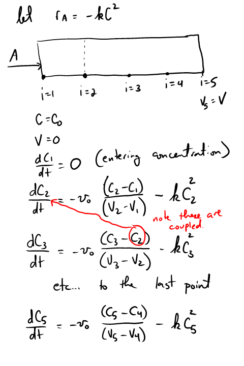
Problem setup

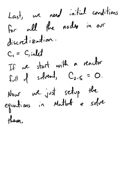
Ca0 = 2; % Entering concentration
vo = 2; % volumetric flow rate
volume = 20;  % total volume of reactor, spacetime = 10
k = 1;  % reaction rate constant

N = 100; % number of points to discretize the reactor volume on

init = zeros(N,1); % Concentration in reactor at t = 0
init(1) = Ca0; % concentration at entrance

V = linspace(0,volume,N)'; % discretized volume elements, in column form

tspan = [0 20];
[t,C] = ode15s(@method_of_lines,tspan,init);

plotting the solution

The solution contains the time dependent behavior of each node in the discretized reactor. For example, we can plot the concentration of A at the exit vs. time as:

plot(t,C(:,end))
xlabel('time')
ylabel('Concentration at exit')

You can see that around the space time, species A breaks through the end of the reactor, and rapidly rises to a steady state value.

animating the solution

It isn't really illustrative to examine only the exit concentration. We can also create an animated gif to show how the concentration of A throughout the reactor varies with time.

filename = 'transient-pfr.gif'; % file to store image in
for i=1:5:length(t) % only look at every 5th time step
    plot(V,C(i,:));
    ylim([0 2])
    xlabel('Reactor volume')
    ylabel('C_A')
    text(0.1,1.9,sprintf('t = %1.2f',t(i))); % add text annotation of time step
    frame = getframe(1);
    im = frame2im(frame); %convert frame to an image
    [imind,cm] = rgb2ind(im,256);

    % now we write out the image to the animated gif.
    if i == 1;
        imwrite(imind,cm,filename,'gif', 'Loopcount',inf);
    else
        imwrite(imind,cm,filename,'gif','WriteMode','append');
    end
end
close all; % makes sure the plot from the loop above doesn't get published

here is the animation!

You can see that the steady state behavior is reached at approximately 10 time units, which is the space time of the reactor in this example.

Add steady state solution

It is good to double check that we get the right steady state behavior. We can solve the steady state plug flow reactor problem like this:

    function dCdV = pfr(V,C)
        dCdV = 1/vo*(-k*C^2);
    end

figure; hold all
vspan = [0 20];
[V_ss Ca_ss] = ode45(@pfr,vspan,2);
plot(V_ss,Ca_ss,'k--','linewidth',2)
plot(V,C(end,:),'r') % last solution of transient part
legend 'Steady state solution' 'transient solution at t=100'

there is some minor disagreement between the final transient solution and the steady state solution. That is due to the approximation in discretizing the reactor volume. In this example we used 100 nodes. You get better agreement with a larger number of nodes, say 200 or more. Of course, it takes slightly longer to compute then, since the number of coupled odes is equal to the number of nodes.

end

% categories: PDEs
% tags: reaction engineering

Published with MATLAB® 7.13

transient heat conduction - partial differential equations

adapated from http://msemac.redwoods.edu/~darnold/math55/DEproj/sp02/AbeRichards/slideshowdefinal.pdf

Contents

In Post 860 we solved a steady state BVP modeling heat conduction. Today we examine the transient behavior of a rod at constant T put between two heat reservoirs at different temperatures, again T1 = 100, and T2 = 200. The rod will start at 150. Over time, we should expect a solution that approaches the steady state solution: a linear temperature profile from one side of the rod to the other.

at , in this example we have as an initial condition. with boundary conditions and .

Matlab provides the pdepe command which can solve some PDEs. The syntax for the command is

 sol = pdepe(m,@pdex,@pdexic,@pdexbc,x,t)

where m is an integer that specifies the problem symmetry. The three function handles define the equations, initial conditions and boundary conditions. x and t are the grids to solve the PDE on.

function pdexfunc

close all; clc; clear all;

setup the problem

m=0; % specifies 1-D symmetry
x = linspace(0,1); % equally-spaced points along the length of the rod
t = linspace(0,5); % this creates time points

sol = pdepe(m,@pdex,@pdexic,@pdexbc,x,t);

plot the solution as a 3D surface

x is the position along the rod, t is the time sol is the temperature at (x,t)

surf(x,t,sol)
xlabel('Position')
ylabel('time')
zlabel('Temperature')

in the surface plot above you can see the approach from the initial conditions to the steady state solution.

we can also plot the solutions in 2D, at different times. Our time vector has about 100 elements, so in this loop we plot every 5th time. We set a DisplayName in each plot so we can use them in the legend later.

figure
hold all % the use of all makes the colors cycle with each plot
for i=1:5:numel(t)
    plot(x,sol(i,:),'DisplayName',sprintf('t = %1.2f',t(i)))
end
xlabel('length')
ylabel('Temperature')

% we use -DynamicLegend to pick up the display names we set above.
legend('-DynamicLegend','location','bestoutside');
% this is not an easy way to see the solution.

animating the solution

we can create an animated gif to show how the solution evolves over time.

filename = 'animated-solution.gif'; % file to store image in
for i=1:numel(t)
    plot(x,sol(i,:));
    xlabel('Position')
    ylabel('Temperature')
    text(0.1,190,sprintf('t = %1.2f',t(i))); % add text annotation of time step
    frame = getframe(1);
    im = frame2im(frame); %convert frame to an image
    [imind,cm] = rgb2ind(im,256);

    % now we write out the image to the animated gif.
    if i == 1;
        imwrite(imind,cm,filename,'gif', 'Loopcount',inf);
    else
        imwrite(imind,cm,filename,'gif','WriteMode','append');
    end
end
close all; % makes sure the plot from the loop above doesn't get published

here is the animation!

It is slightly more clear that the temperature profile evolves from a flat curve, to a linear temperature ramp between the two end points.

'done'

ans =

done

function [c,f,s] = pdex(x,t,u,DuDx)

For pdepe to understand the equations, they need to be in the form of

where c is a diagonal matrix, f is called a flux term, and s is the source term. Our equations are:

from which you can see that , , and

c = 1;
f = 0.02*DuDx;
s = 0;

function u0 = pdexic(x)
% this defines u(t=0) for all of x. The problem specifies a constant T for
% all of x.
u0 = 150;

function [p1,q1,pr,qr] = pdexbc(x1,u1,xr,ur,t)
% this defines the boundary conditions. The general form of the boundary
% conditions are $p(x,t,u) + q(x,t)f(x,t,u,\frac{\partial u}{\partial x})$
% We have to define the boundary conditions on the left, and right.
p1 = u1-100; % at left
q1 = 0; % at left
pr= ur-200;  % at right
qr = 0; % at right


% categories: PDEs
% tags: heat transfer

Published with MATLAB® 7.10