On the quad, or trapz'd in ChemE heaven?

| categories: basic matlab | View Comments

on_the_quad

Contents

On the quad, or trapz'd in ChemE heaven?

John Kitchin

What is the difference between quad and trapz? The short answer is that quad integrates functions (via a function handle) using numerical quadrature, and trapz performs integration of arrays of data using the trapezoid method.

Let's look at some examples. We consider the example of computing $\int_0^2 x^3 dx$. the analytical integral is $1/4 x^4$, so we know the integral evaluates to 16/4 = 4. This will be our benchmark for comparison to the numerical methods.

clear all; clc; close all;

quad usage

This command is equivalent to $\int_0^2 x^3 dx$

i1 = quad(@(x) x.^3,0,2)
i1 =

     4

we can also define the function handle separately.

f = @(x) x.^3
f(2) % should be 8
f = 

    @(x)x.^3


ans =

     8

This command is equivalent to $\int_0^2 f(x) dx$

i1 = quad(f,0,2)
error = (i1 - 4)/4
% Note the error is very small!
i1 =

     4


error =

     0

Trapz usage

if we had numerical data like this, we use trapz to integrate it

x = [0 0.5 1 1.5 2];
y = f(x);  % or you could say y = x.^3

i2 = trapz(x,y)
error = (i2 - 4)/4
i2 =

    4.2500


error =

    0.0625

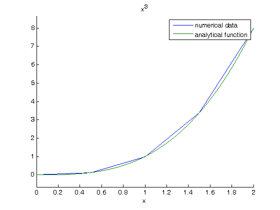
Note the integral of these vectors is greater than 4! You can see why here.

figure; hold all
plot(x,y)
ezplot(f,[0 2])
legend 'numerical data' 'analytical function'
% The area of the trapezoids is greater than the area under the function
% due to the coarse sampling of $f(x)=x^3$.

with a finer sampling we have:

x = linspace(0,2); % 100 points between 0, 1
y = x.^3;
i3 = trapz(x,y)
i3 =

    4.0004

and a much smaller error.

error = (i3 - 4)/4
error =

  1.0203e-004

Combining numerical data with quad

You might want to combine numerical data with the quad function if you want to perform integrals easily. Let's say you are given this data:

x = [0 0.5 1 1.5 2];
y = [0    0.1250    1.0000    3.3750    8.0000];

and you want to integrate this from x = 0.25 to 1.75. We don't have data in those regions, so some interpolation is going to be needed. Here is the analytical integral and by numerical quadrature

i_analytical = 1/4*(1.75^4-0.25^4)
i = quad(f,0.25,1.75)
% they are practically the same.
i_analytical =

    2.3438


i =

    2.3437

One way to do this with the data provided is to use interpolation on a fine-spaced x-grid, and then use trapz on the resulting interpolated vectors.

xfine = linspace(0.25,1.75);
yinterp = interp1(x,y,xfine);
i4 = trapz(xfine,yinterp)
error = (i4 - i_analytical)/i_analytical
i4 =

    2.5315


error =

    0.0801

Another approach is to create a function handle to do the interpolation for you. This combines numerical data with the quad function!

finterp = @(X) interp1(x,y,X);
i5 = quad(finterp,0.25,1.75)
error = (i5 - i_analytical)/i_analytical
i5 =

    2.5312


error =

    0.0800

these two approaches are actually identical, as they are both based on linear interpolation. The second approach is slightly more compact and easier to evaluate multiple integrals. Compare:

i6 = quad(finterp,0.28,1.64)
i6 =

    1.9596

to:

xfine = linspace(0.28,1.64);
yinterp = interp1(x,y,xfine);
i7 = trapz(xfine,yinterp)
% One line of code vs. three.
i7 =

    1.9597

Summary

trapz and quad are functions for getting integrals. Both can be used with numerical data if interpolation is used.

Finally, see this post for an example of solving an integral equation using quad and fsolve.

% categories: basic matlab
% tags: integration
Read and Post Comments

The equal area method for the van der Waals equation

| categories: nonlinear algebra | View Comments

The equal area method for the van der Waals equation

The equal area method for the van der Waals equation

John Kitchin

Contents

Introduction

When a gas is below its Tc the van der Waal equation oscillates. In the portion of the isotherm where $\partial P_R/\partial V_r > 0$, the isotherm fails to describe real materials, which phase separate into a liquid and gas in this region.

Maxwell proposed to replace this region by a flat line, where the area above and below the curves are equal. Today, we examine how to identify where that line should be.

function maxwell_equal_area_2
clc; clear all; close all

Tr = 0.9; % A Tr below Tc:  Tr = T/Tc
% analytical equation for Pr. This is the reduced form of the van der Waal
% equation.
Prfh = @(Vr) 8/3*Tr./(Vr - 1/3) - 3./(Vr.^2);

Vr = linspace(0.5,4,100);   % vector of reduced volume
Pr = Prfh(Vr);              % vector of reduced pressure

Plot the vdW EOS

figure; hold all
plot(Vr,Pr)
ylim([0 2])
xlabel('V_R')
ylabel('P_R')

show unstable region

dPdV = cmu.der.derc(Vr, Pr);
plot(Vr(dPdV > 0),Pr(dPdV > 0),'r-','linewidth',2)

Idea behind Maxwell equal area principle

The idea is to pick a Pr and draw a line through the EOS. We want the areas between the line and EOS to be equal on each side of the middle intersection.

y = 0.65;  % Pr that defines the horizontal line
plot([0.5 4],[y y],'k--') % horizontal line

find three roots

To find the areas, we need to know where the intersection of the vdW eqn with the horizontal line. This is the same as asking what are the roots of the vdW equation at that Pr. We need all three intersections so we can integrate from the first root to the middle root, and then the middle root to the third root. We take advantage of the polynomial nature of the vdW equation, which allows us to use the roots command to get all the roots at once. The polynomial is $V_R^3 - \frac{1}{3}(1+8 T_R/P_R) + 3/P_R - 1/P_R = 0$. We use the coefficients t0 get the rooys like this.

vdWp = [1 -1/3*(1+8*Tr/y) 3/y -1/y];
v = sort(roots(vdWp))
v =

    0.6029
    1.0974
    2.3253

plot the roots

we want to make sure the roots are really the intersections with the line.

plot(v(1),y,'bo',v(2),y,'bo',v(3),y,'bo')

compute areas

for A1, we need the area under the line minus the area under the vdW curve. That is the area between the curves. For A2, we want the area under the vdW curve minus the area under the line. The area under the line between root 2 and root 1 is just the width (root2 - root1)*y

A1 = (v(2)-v(1))*y - quad(Prfh,v(1),v(2))
A2 = quad(Prfh,v(2),v(3)) - (v(3)-v(2))*y
% these areas are pretty close, and we could iterate to get them very
% close. or, we can use a solver to do this. To do that, we need to define
% a function that is equal to zero when the two areas are equal. See the
% equalArea function below.

Pr_equal_area = fzero(@equalArea, 0.65)
A1 =

    0.0632


A2 =

    0.0580


Pr_equal_area =

    0.6470

confirm the two areas are equal

y = Pr_equal_area;
equalArea(y) % this should be close to zero
ans =

  1.1102e-016

and we can compute the areas too

vdWp = [1 -1/3*(1+8*Tr/y) 3/y -1/y]
v = sort(roots(vdWp))
A1 = (v(2)-v(1))*y - quad(Prfh,v(1),v(2))
A2 = quad(Prfh,v(2),v(3)) - (v(3)-v(2))*y
% these areas are very close to each other.
vdWp =

    1.0000   -4.0428    4.6368   -1.5456


v =

    0.6034
    1.0905
    2.3488


A1 =

    0.0618


A2 =

    0.0618

plot the areas that are equal

we want to show the areas that are equal by shading them.

xx = [v(1) Vr(Vr >= v(1) & Vr <= v(2)) v(2)];
yy = [Prfh(v(1)) Pr(Vr >= v(1) & Vr <= v(2)) Prfh(v(2))];
lightgray = [0.9 0.9 0.9];
fill(xx,yy,lightgray)

xx = [v(2) Vr(Vr >= v(2) & Vr <= v(3)) v(3)];
yy = [Prfh(v(2)) Pr(Vr >= v(2) & Vr <= v(3)) Prfh(v(3))];
fill(xx,yy,lightgray)
% and finally lets add text labels to the figure for what the areas are.
text(v(1),1,sprintf('A1 = %f',A1))
text(v(3),1,sprintf('A2 = %f',A2))

Finally, plot the isotherm

we want to replace the unstable region with the flat line that defines the equal areas. The roots are stored in the variable $v$
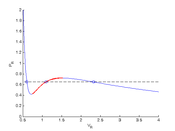
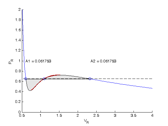
. We use logical indexing to select the parts of the data that we want.

figure
Vrf = [Vr(Vr <= v(1)) v(1)       v(3)       Vr(Vr>= v(3))];
Prf = [Pr(Vr <= v(1)) Prfh(v(1)) Prfh(v(3)) Pr(Vr>= v(3))];
plot(Vrf,Prf)
ylim([0 2])
xlabel('V_R')
ylabel('P_R')
title('T_R = 0.9')

The flat line in this isotherm corresponds to a vapor-liquid equilibrium. This is the result for $T_R = 0.9$
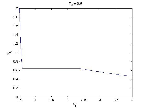
. You could also compute the isotherm for other $T_R$ values.

'done'
ans =

done

function Z = equalArea(y)
% compute A1 - A2 for Tr = 0.9.
Tr = 0.9;
vdWp = [1 -1/3*(1+8*Tr/y) 3/y -1/y];
v = sort(roots(vdWp));

Prfh = @(Vr) 8/3*Tr./(Vr - 1/3) - 3./(Vr.^2);
A1 = (v(2)-v(1))*y - quad(Prfh,v(1),v(2));
A2 = quad(Prfh,v(2),v(3)) - (v(3)-v(2))*y;

Z = A1 - A2;

% categories: Nonlinear algebra
% tags: thermodynamics
Read and Post Comments

Counting roots

| categories: odes, nonlinear algebra | View Comments

Counting roots

Counting roots

John Kitchin

Contents

Problem statement

The goal here is to determine how many roots there are in a nonlinear function we are interested in solving. For this example, we use a cubic polynomial because we know there are three roots.

$$f(x) = x^3 + 6x^2 - 4x -24$$

function main
clc; clear all; close all;

Use roots for this polynomial

This ony works for a polynomial, it does not work for any other nonlinear function.

roots([1 6 -4 -24])
ans =

   -6.0000
    2.0000
   -2.0000

Plot the function to see where the roots are

x = linspace(-8,4);
fx = x.^3 + 6*x.^2 - 4*x - 24;
plot(x,fx)

method 1

count the number of times the sign changes in the interval. We determine the sign of each element (-1, 0 or +1) and then use a a loop to go through each element. A sign change is detected when an element is not equal to the previous element. Note this is not foolproof; we may over count roots if we get a sequence -1 0 1. We check for that by making sure neither of the two elements being compared are zero.

sign_fx = sign(fx);

count = 0;
for i=2:length(sign_fx)
    if sign_fx(i) ~= sign_fx(i-1) && sign_fx(i) ~= 0 && sign_fx(i-1) ~= 0
        count = count + 1;
        disp(sprintf('A root is between x = %f and %f',x(i-1),x(i)))
    end
end

disp(sprintf('The number of sign changes is %i.',count))
A root is between x = -6.060606 and -5.939394
A root is between x = -2.060606 and -1.939394
A root is between x = 1.939394 and 2.060606
The number of sign changes is 3.

method 1a

this one line code also counts sign changes. the diff command makes all adjacent, identical elements equal zero, and sign changes = 2 (1 - (-1)) or (-1 - 1). Then we just sum up the diff vector, divide by two, and that is the number of roots. Note that no check for 0 is needed; you will get 1/2 a sign change from -1 to 0. and another half from 0 to 1. They add up to a whole sign change.

sum(abs(diff(sign_fx))/2)
ans =

     3

Discussion

Method 1 is functional but requires some programming. Method 1a is concise but probably tricky to remember.

Method 2

using events in an ODE solver Matlab can identify events in the solution to an ODE, for example, when a function has a certain value, e.g. f(x) = 0. We can take advantage of this to find the roots and number of roots in this case.

$$f'(x) = 3x^2 + 12x - 4$$

with f(-8) = -120

xspan = [-8 4];
fp0 = -120;

options = odeset('Events',@event_function);
[X,Y,XE,VE,IE] = ode45(@myode,xspan,fp0,options);
XE % these are the x-values where the function equals zero
nroots = length(XE);
disp(sprintf('Found %i roots in the x interval',nroots))

% lets compare the solution to the  original function to make sure they are
% the same.
figure
plot(X,Y,x,fx)
legend 'numerical' 'analytical'
function dfdx = myode(x,f)
dfdx = 3*x^2 + 12*x - 4;

function [value,isterminal,direction] = event_function(t,y)
value = y - 0;  % then value = 0, an event is triggered
isterminal = 0; % do not terminate after the first event
direction = 0;  % get all the zeros

% categories: ODEs, nonlinear algebra
XE =

   -6.0000
   -2.0000
    2.0000

Found 3 roots in the x interval
Read and Post Comments

Reading parameter database text files in Matlab

| categories: file io | View Comments

read_use_antoine

Contents

Reading parameter database text files in Matlab

John Kitchin

clear all; clc; close all

the datafile at http://terpconnect.umd.edu/~nsw/ench250/antoine.dat contains data that can be used to estimate the vapor pressure of about 700 pure compounds using the Antoine equation

The data file has the following contents:

 Antoine Coefficients
   log(P) = A-B/(T+C) where P is in mmHg and T is in Celsius
 Source of data: Yaws and Yang (Yaws, C.  L.  and Yang, H.  C.,
 "To estimate vapor pressure easily. antoine coefficients relate vapor pressure to temperature for almost 700 major organic compounds", Hydrocarbon Processing, 68(10), p65-68, 1989.
 ID  formula  compound name                  A       B       C     Tmin Tmax ??    ?
 -----------------------------------------------------------------------------------
   1 CCL4     carbon-tetrachloride        6.89410 1219.580 227.170  -20  101 Y2    0
   2 CCL3F    trichlorofluoromethane      6.88430 1043.010 236.860  -33   27 Y2    0

To use this data, you find the line that has the compound you want, and read off the data. You could do that manually for each component you want but that is tedious, and error prone. Today we will see how to retrieve the file, then read the data into Matlab to create a database we can use to store and retrieve the data.

We will use the data to find the temperature at which the vapor pressure of acetone is 400 mmHg.

get a local copy of the file

urlwrite('http://terpconnect.umd.edu/~nsw/ench250/antoine.dat','antoine_data.dat');

Reading in the data

We use the textscan command to skip the first 7 header lines, and then to parse each line according to the format string. After the header, each line has the format of:

 integer string string float float float float float string string

which we represent by '%d%s%s%f%f%f%f%f%s%s' as a format string. Note we are basically ignoring the contents of the last two columns, and just reading them in as strings. The output of the textread command will be a vector of values for each numerical column, and a cell array for string data.

now open it, and read it

the output of the textscan command is a cell array of all the data read in.

fid = fopen('antoine_data.dat');
C = textscan(fid,'%d%s%s%f%f%f%f%f%s%s','headerlines',7);
fclose(fid);

convert the cell array output of textscan into variables

This makes it easier to read the code where we assign the database. Each of these varialbes is a column vector containing the data for that column in our text file.

[id formula compound A B C Tmin Tmax i j] = C{:};

the database

the Map object will let us refer to an entry as database('acetone')

database = containers.Map();

storing the data

for i=1:length(id)
    % we store the data as a cell for each compound
    database(compound{i}) = {A(i) B(i) C(i) Tmin(i) Tmax(i)};
end
% That's it! Now, we can use the database to retrieve specific entries.

Now use the database to plot the vapor pressure of acetone

get the parameters for acetone

compound = database('acetone')
% for readability let's pull out each data property into variable names
[A B C Tmin Tmax] = compound{:}
compound = 

    [7.2316]    [1.2770e+003]    [237.2300]    [-32]    [77]


A =

    7.2316


B =

  1.2770e+003


C =

  237.2300


Tmin =

   -32


Tmax =

    77

plot vapor pressure of acetone over the allowable temperature range.

T = linspace(Tmin, Tmax);
P = 10.^(A - B./(T+C));
plot(T,P)
xlabel('T (\circC)')
ylabel('P_{vap} (mmHg)')

Find T at which Pvap = 400 mmHg

from our graph we might guess T ~ 40 degC

Tguess = 40;
f = @(T) 400 - 10.^(A - B./(T+C));
T400 = fzero(f,Tguess)

sprintf('The vapor pressure is 400 mmHg at T = %1.1f degC',T400)
T400 =

   38.6138


ans =

The vapor pressure is 400 mmHg at T = 38.6 degC

This result is close to the value reported here (39.5 degC), from the CRC Handbook. The difference is probably that the value reported in the CRC is an actual experimental number.

Plot CRC data

We only include the data for the range where the Antoine fit is valid.

T  = [-59.4 	-31.1 	-9.4 	7.7 	39.5 	56.5];
P = [	1 	10 	40 	100 	400 	760];

hold all
plot(T,P,'bo')
legend('Antoine','CRC Handbook','location','northwest')
% There is pretty good agreement between the Antoine equation and the data.

save the database for later use.

we can load this file into Matlab at a later time instead of reading in the text file again.

save  antoine_database.mat database

% categories: File IO
% tags: thermodynamics
Read and Post Comments

Plane Poiseuille flow - BVP solve by shooting method

| categories: odes | View Comments

Plane Poiseuille flow - BVP solve by shooting method

Plane Poiseuille flow - BVP solve by shooting method

In Post 878 learned how to use the BVP solver in Matlab to solve a boundary value problem. Another approach is to use the shooting method. The reason we can't use an initial value solver for a BVP is that there is not enough information at the initial value to start. In the shooting method, we take the function value at the initial point, and guess what the function derivatives are so that we can do an integration. If our guess was good, then the solution will go through the known second boundary point. If not, we guess again, until we get the answer we need. In this example we repeat the pressure driven flow example, but illustrate the shooting method.

In the pressure driven flow of a fluid with viscosity $\mu$ 
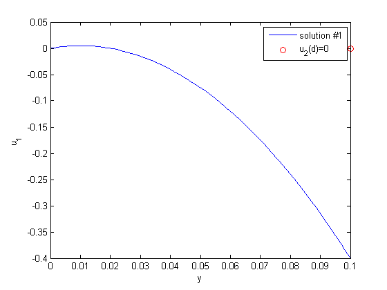
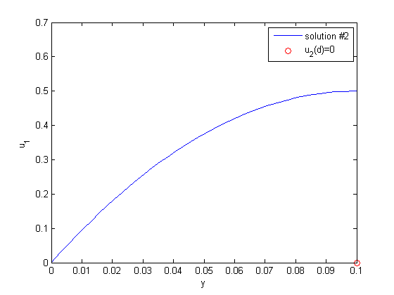
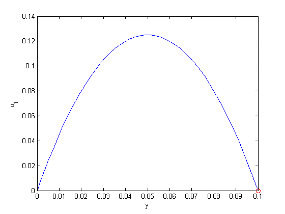
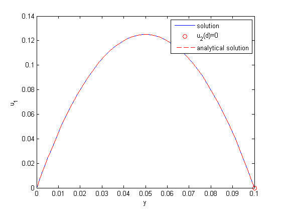
between two stationary plates separated by distance $d$ and driven by a pressure drop $\Delta P/\Delta x$, the governing equations on the velocity $u$ of the fluid are (assuming flow in the x-direction with the velocity varying only in the y-direction):

Contents

$$\frac{\Delta P}{\Delta x} = \mu \frac{d^2u}{dy^2}$$

with boundary conditions $u(y=0) = 0$ and $u(y=d) = 0$, i.e. the no-slip condition at the edges of the plate.

we convert this second order BVP to a system of ODEs by letting $u_1 = u$, $u_2 = u_1'$ and then $u_2' = u_1''$. This leads to:

$\frac{d u_1}{dy} = u_2$

$\frac{d u_2}{dy} = \frac{1}{\mu}\frac{\Delta P}{\Delta x}$

with boundary conditions $u_1(y=0) = 0$ and $u_1(y=d) = 0$.

for this problem we let the plate separation be d=0.1, the viscosity $\mu = 1$, and $\frac{\Delta P}{\Delta x} = -100$.

function main
clc; close all; clear all;

d = 0.1; % plate thickness

First guess

we need u_1(0) and u_2(0), but we only have u_1(0). We need to guess a value for u_2(0) and see if the solution goes through the u_2(d)=0 boundary value.

u1_0 = 0; % known
u2_0 = 1; % guessed

init = [u1_0 u2_0];
dspan = [0 d];
[y,U] = ode45(@odefun,dspan,init);
plot(y,U(:,1),[d],[0],'ro')
legend 'solution #1' 'u_2(d)=0'
xlabel('y')
ylabel('u_1')
% It appears we have undershot, so our initial slope was not large
% enough

second guess

u1_0 = 0; % known
u2_0 = 10; % guessed

init = [u1_0 u2_0];
dspan = [0 d];
[y,U] = ode45(@odefun,dspan,init);
plot(y,U(:,1),[d],[0],'ro')
legend 'solution #2' 'u_2(d)=0'
xlabel('y')
ylabel('u_1')
% Now we have overshot, the initial slope is too high. The right
% answer must be between 1 and 10 You could continue to iterate on
% this manually until the value of u_1(d) = 0. Instead, we use a
% solver to do that, now that we have a reasonable guess for u_2(0).

Using a solver

we have to make a function that is equal to zero when u_2(d) = 0.

u2_guess = 2;
u2_0_solved = fsolve(@myfunc,u2_guess)
Equation solved.

fsolve completed because the vector of function values is near zero
as measured by the default value of the function tolerance, and
the problem appears regular as measured by the gradient.


u2_0_solved =

    5.0000

Plot final solution

init = [u1_0 u2_0_solved];
dspan = [0 d];
[y,U] = ode45(@odefun,dspan,init);

figure
plot(y,U(:,1),d,0,'ro')
xlabel('y')
ylabel('u_1')

Known analytical solution

the analytical solution to this problem is known, and we can plot it on top of the numerical solution

mu = 1;
Pdrop = -100; % this is DeltaP/Deltax
u = -(Pdrop)*d^2/2/mu*(y/d-(y/d).^2);
hold all
plot(y,u,'r--')
legend 'solution' 'u_2(d)=0' 'analytical solution'
'done'
ans =

done

Finally, the solutions agree, and show that the velocity profile is parabolic, with a maximum in the middle of the two plates. You can also see that the velocity at each boundary is zero, as required by the boundary conditions

function dUdy = odefun(y,U)
% here we define our differential equations
u1 = U(1);
u2 = U(2);

mu = 1;
Pdrop = -100; % this is DeltaP/Deltax
du1dy = u2;
du2dy = 1/mu*Pdrop;
dUdy = [du1dy; du2dy];


function Z = myfunc(u2_guess)
% this function is zero when u_1(d) = 0.
u1_0 = 0; % known
u2_0 = u2_guess; % guessed
d = 0.1;

init = [u1_0 u2_0];
dspan = [0 d];
sol = ode45(@odefun,dspan,init);

u = deval(sol,d); % u = [u_1(d) u_2(d)]
u1_d = u(1);
Z = u1_d;

% categories: ODEs
% tags: math, fluids, bvp


% post_id = 1036; %delete this line to force new post;
Read and Post Comments

« Previous Page -- Next Page »