Solving an ode for a specific solution value
August 31, 2011 at 08:01 PM | categories: odes | View Comments
Solving an ode for a specific solution value
John Kitchin 8/31/2011
The analytical solution to an ODE is a function, which can be solved to get a particular value, e.g. if the solution to an ODE is y(x) = exp(x), you can solve the solution to find the value of x that makes  . In a numerical solution to an ODE we get a vector of independent variable values, and the corresponding function values at those values. To solve for a particular function value we need a different approach. This post will show one way to do that in Matlab.
Contents
The problem
given that the concentration of a species A in a constant volume, batch reactor obeys this differential equation  with the initial condition
 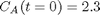 mol/L and
  L/mol/s, compute the time it takes for
  to be reduced to 1 mol/L.
Solution
we will use Matlab to integrate the ODE to obtain the solution, and then use the deval command in conjuction with fsolve to get the numerical solution we are after.
clear all; close all; clc

k = 0.23;
Cao = 2.3;
dCadt = @(t,Ca) -k*Ca^2;
tspan = [0 10];
sol = ode45(dCadt,tspan,Cao)
% sol here is a struct with fields corresponding to the solution and other
% outputs of the solver.
sol =

     solver: 'ode45'
    extdata: [1x1 struct]
          x: [1x12 double]
          y: [1x12 double]
      stats: [1x1 struct]
      idata: [1x1 struct]
We need to make sure the solution vector from the ode solver contains the answer we need
plot(sol.x,sol.y)
xlabel('Time (s)')
ylabel('C_A (mol/L)')
% the concentration of A is at approximately t=3
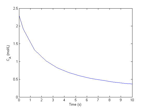
We can make a function Ca(t) using the solution from the ode solver and the deval command, which evaluates the ODE solution at a new value of t.
Ca = @(t) deval(sol,t);

% now we create a function for fsolve to work on. remember this function is
% equal to zero at the solution.
tguess = 3;
f = @(t) 1 - Ca(t) ;
t_solution = fsolve(f,tguess)

Ca(t_solution) % this should be 1.0

sprintf('C_A = 1 mol/L at a time of %1.2f seconds.',t_solution)
Equation solved.

fsolve completed because the vector of function values is near zero
as measured by the default value of the function tolerance, and
the problem appears regular as measured by the gradient.


t_solution =

    2.4598


ans =

    1.0000


ans =

C_A = 1 mol/L at a time of 2.46 seconds.
A related post is Post 954 on solving integral equations.
'done'

% categories: ODEs
% tags: reaction engineering
% post_id = 968; %delete this line to force new post;
ans =

done
 where
where  is the rate law. Suppose we know the reactor volume is 100 L, the inlet molar flow of A is 1 mol/L, the volumetric flow is 10 L/min, and
  , with
  1/min. What is the exit molar flow rate? We need to solve the following equation:


![$A = \left[ \begin{array}{cc} -1 & 0 \\ 0 & -1 \\ 1 & 1 \end{array} \right]$](http://matlab.cheme.cmu.edu/wp-content/uploads/2011/08/Gmin_eq10921.png) and
and ![$b = \left[ \begin{array}{c} 0 \\ 0 \\ 0.5\end{array} \right]$](http://matlab.cheme.cmu.edu/wp-content/uploads/2011/08/Gmin_eq62028.png)