Numerically calculating an effectiveness factor for a porous catalyst bead

| categories: bvp | View Comments

effectiveness_factor

Contents

Numerically calculating an effectiveness factor for a porous catalyst bead

John Kitchin

If reaction rates are fast compared to diffusion in a porous catalyst pellet, then the observed kinetics will appear to be slower than they really are because not all of the catalyst surface area will be effectively used. For example, the reactants may all be consumed in the near surface area of a catalyst bead, and the inside of the bead will be unutilized because no reactants can get in due to the high reaction rates.

References: Ch 12. Elements of Chemical Reaction Engineering, Fogler, 4th edition.

function  main
close all; clc; clear all

The governing equations for reaction and diffusion

A mole balance on the particle volume in spherical coordinates with a first order reaction leads to: $\frac{d^2Ca}{dr^2} + \frac{2}{r}\frac{dCa}{dr}-\frac{k}{D_e}C_A=0$ with boundary conditions $C_A(R) = C_{As}$ and $\frac{dCa}{dr}=0$ at $r=0$. We convert this equation to a system of first order ODEs by letting $W_A=\frac{dCa}{dr}$.

    function dYdt = ode(r,Y)

        Wa = Y(1); % molar rate of delivery of A to surface of particle
        Ca = Y(2); % concentration of A in the particle at r

        if r == 0
            dWadr = 0; % this solves the singularity at r = 0
        else
            dWadr = -2*Wa/r + k/De*Ca;
        end

        dCadr = Wa;

        dYdt = [dWadr; dCadr];
    end

Parameters for this problem

De = 0.1;   % diffusivity cm^2/s
R = 0.5;    % particle radius, cm
k = 6.4;    % rate constant (1/s)
CAs = 0.2;  % concentration of A at outer radius of particle (mol/L)

Solving the BVP

we have a condition of no flux at r=0 and Ca® = CAs, which makes this a boundary value problem. We use the shooting method here, and guess what Ca(0) is and iterate the guess to get Ca® = CAs.

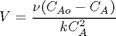
Ca0 = 0.029315; % Ca(0) (mol/L) guessed to satisfy Ca(R) = CAs
Wa0 = 0;    % no flux at r=0 (mol/m^2/s)
init = [Wa0 Ca0];
rspan = [0 R];

[r Y] = ode45(@ode,rspan, init);
Ca = Y(:,2);

plot(r,Ca)
xlabel('Particle radius')
ylabel('C_A')

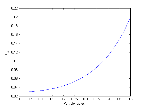
You can see the concentration of A inside the particle is significantly lower than outside the particle. That is because it is reacting away faster than it can diffuse into the particle. Hence, the overall reaction rate in the particle is lower than it would be without the diffusion limit.

Compute the effectiveness factor numerically

The effectiveness factor is the ratio of the actual reaction rate in the particle with diffusion limitation to the ideal rate in the particle if there was no concentration gradient:

$$\eta = \frac{\int_0^R k'' a C_A(r) 4 \pi r^2 dr}{\int_0^R k'' a
C_{As} 4 \pi r^2 dr}$$

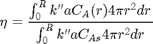
We will evaluate this numerically from our solution.

eta_numerical = trapz(r, k*Ca*4*pi.*(r.^2))/trapz(r, k*CAs*4*pi.*(r.^2))
eta_numerical =

    0.5635

Analytical solution for a first order reaction

an analytical solution exists for this problem.

phi = R*sqrt(k/De);
eta = (3/phi^2)*(phi*coth(phi)-1)
eta =

    0.5630

Why go through the numerical solution when an analytical solution exists? The analytical solution here is only good for 1st order kinetics in a sphere. What would you do for a complicated rate law? You might be able to find some limiting conditions where the analytical equation above is relevant, and if you are lucky, they are appropriate for your problem. If not, it's a good thing you can figure this out numerically!

end

% categories: BVP
% tags: reaction engineering
Read and Post Comments

Modeling a transient plug flow reactor

| categories: pdes | View Comments

Modeling a transient plug flow reactor

Modeling a transient plug flow reactor

John Kitchin

Contents

function main
clear all; clc; close all

    function dCdt = method_of_lines(t,C)
        % we use vectorized operations to define the odes at each node
        % point.
        dCdt = [0; % C1 does not change with time, it is the entrance of the pfr
               -vo*diff(C)./diff(V)-k*C(2:end).^2];
    end

Problem setup

Ca0 = 2; % Entering concentration
vo = 2; % volumetric flow rate
volume = 20;  % total volume of reactor, spacetime = 10
k = 1;  % reaction rate constant

N = 100; % number of points to discretize the reactor volume on

init = zeros(N,1); % Concentration in reactor at t = 0
init(1) = Ca0; % concentration at entrance

V = linspace(0,volume,N)'; % discretized volume elements, in column form

tspan = [0 20];
[t,C] = ode15s(@method_of_lines,tspan,init);

plotting the solution

The solution contains the time dependent behavior of each node in the discretized reactor. For example, we can plot the concentration of A at the exit vs. time as:

plot(t,C(:,end))
xlabel('time')
ylabel('Concentration at exit')

You can see that around the space time, species A breaks through the end of the reactor, and rapidly rises to a steady state value.

animating the solution

It isn't really illustrative to examine only the exit concentration. We can also create an animated gif to show how the concentration of A throughout the reactor varies with time.

filename = 'transient-pfr.gif'; % file to store image in
for i=1:5:length(t) % only look at every 5th time step
    plot(V,C(i,:));
    ylim([0 2])
    xlabel('Reactor volume')
    ylabel('C_A')
    text(0.1,1.9,sprintf('t = %1.2f',t(i))); % add text annotation of time step
    frame = getframe(1);
    im = frame2im(frame); %convert frame to an image
    [imind,cm] = rgb2ind(im,256);

    % now we write out the image to the animated gif.
    if i == 1;
        imwrite(imind,cm,filename,'gif', 'Loopcount',inf);
    else
        imwrite(imind,cm,filename,'gif','WriteMode','append');
    end
end
close all; % makes sure the plot from the loop above doesn't get published

here is the animation!

You can see that the steady state behavior is reached at approximately 10 time units, which is the space time of the reactor in this example.

Add steady state solution

It is good to double check that we get the right steady state behavior. We can solve the steady state plug flow reactor problem like this:

    function dCdV = pfr(V,C)
        dCdV = 1/vo*(-k*C^2);
    end

figure; hold all
vspan = [0 20];
[V_ss Ca_ss] = ode45(@pfr,vspan,2);
plot(V_ss,Ca_ss,'k--','linewidth',2)
plot(V,C(end,:),'r') % last solution of transient part
legend 'Steady state solution' 'transient solution at t=100'

there is some minor disagreement between the final transient solution and the steady state solution. That is due to the approximation in discretizing the reactor volume. In this example we used 100 nodes. You get better agreement with a larger number of nodes, say 200 or more. Of course, it takes slightly longer to compute then, since the number of coupled odes is equal to the number of nodes.

end

% categories: PDEs
% tags: reaction engineering
Read and Post Comments

Parameterized ODEs

| categories: odes | View Comments

Parameterized ODEs

Parameterized ODEs

John Kitchin

Sometimes we have an ODE that depends on a parameter, and we want to solve the ODE for several parameter values. It is inconvenient to write an ode function for each parameter case. Here we examine a convenient way to solve this problem. We consider the following ODE:

Contents

$$\frac{dCa}{dt} = -k Ca(t)$$

where $k$ 
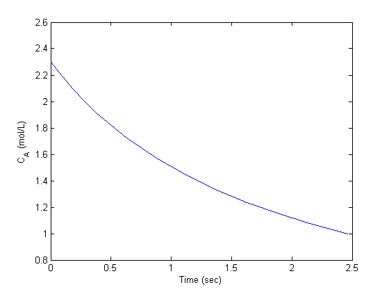
is a parameter, and we want to solve the equation for a couple of values of $k$ to test the sensitivity of the solution on the parameter. Our question is, given $Ca(t=0)=2$, how long does it take to get $Ca = 1$, and how sensitive is the answer to small variations in $k$?

function main
clear all; close all; clc
ko = 2;
tspan = [0 1]; % you need to make sure this time span contains the solution!
Cao = 2;

finding the solution

we will use an events function to make the integration stop where we want it to. First we create an options variable for our ode solver to use the event function to stop integrating at Ca = 1

options = odeset('Events',@event_function);

we will look at +- 5% of the given k-value

ktest = [0.95*ko ko 1.05*ko]
results = [];
ktest =

    1.9000    2.0000    2.1000

this syntax loops through each value in ktest, setting the kvar variable equal to that value inside the loop.

for kvar = ktest
    % make a function handle using the k for this iteration
    f = @(t,Ca) myode(t,Ca,kvar);
    [t,Ca,TE,VE] = ode45(f, tspan, Cao,options);
    % TE is the time at which Ca = 1
    results = [results TE] % store time for later analysis
    plot(t,Ca,'displayname',sprintf('k = %1.2f',kvar))
    hold all
end

legend('-DynamicLegend')
xlabel('Time')
ylabel('C_A')
results =

    0.3648


results =

    0.3648    0.3466


results =

    0.3648    0.3466    0.3301

sprintf('k = %1.2f:  Ca = 1 at %1.2f time units\n',[ktest;results])
ans =

k = 1.90:  Ca = 1 at 0.36 time units
k = 2.00:  Ca = 1 at 0.35 time units
k = 2.10:  Ca = 1 at 0.33 time units


compute errors

we can compute a percent difference for each variation. We assume that ko is the reference point

em = (results(1) - results(2))/results(2)*100
ep = (results(3) - results(2))/results(2)*100
% We see roughly +-5% error for a 5% variation in the parameter. You
% would have to apply some engineering judgement to determine if that
% is sufficiently accurate.
em =

    5.2632


ep =

   -4.7619

function dCadt = myode(t,Ca,k)
dCadt = -k*Ca;

function [value,isterminal,direction] = event_function(t,Ca)
value = Ca - 1.0;  % when value = 0, an event is triggered
isterminal = 1; % terminate after the first event
direction = 0;  % get all the zeros

% categories: ODEs
% tags: reaction engineering
Read and Post Comments

Know your tolerance

| categories: nonlinear algebra | View Comments

Know your tolerance

Know your tolerance

Given:

Contents

$$V = \frac{\nu (C_{Ao} - C_A)}{k C_A^2}$$

with the information given below, solve for the exit concentration. This should be simple. We use the units package to make sure we don't miss any units.

clear all; close all; clc
u = cmu.units;

Cao = 2*u.mol/u.L;
V = 10*u.L;
nu = 0.5*u.L/u.s;
k = 0.23 * u.L/u.mol/u.s;

function we need to solve

f = @(Ca) V - nu*(Cao - Ca)./(k*Ca.^2);

plot the function to estimate the solution

c = linspace(0,2)*u.mol/u.L;
plot(c/(u.mol/u.L),f(c))
ylim([-0.1 0.1]) % limit the y-range to see the zero easier
xlabel('C_A')
ylabel('f(C_A)')
% we want the value of C_A that makes f(C_A)=0. this happens around C_A=0.5
cguess = 0.5*u.mol/u.L;
c = fsolve(f,cguess)
% it is a little weird that the solution is the same as our initial guess.
% Usually the answer is at least a little different!
Equation solved at initial point.

fsolve completed because the vector of function values at the initial point
is near zero as measured by the default value of the function tolerance, and
the problem appears regular as measured by the gradient.


ans =

  500.0000


Equation solved at initial point.

fsolve completed because the vector of function values at the initial point
is near zero as measured by the default value of the function tolerance, and
the problem appears regular as measured by the gradient.


500/m^3*mol

check your solution

z = f(c)
z.as(u.L)
% this is not really that close to zero, especially when you look at the
% units in L!
-0.00304348*m^3

ans =

-3.043*L

closer look at fsolve

Let's output some more information.

options = optimset('Display','iter');
[X,FVAL,EXITFLAG,OUTPUT] = fsolve(f,cguess,options)
% It should be a warning that zero iterations were taken! Our guess was
% probably not that good! The EXITFLAG=1 means the function ended ok as far
% as fsolve is concerned.
                                         Norm of      First-order   Trust-region
 Iteration  Func-count     f(x)          step         optimality    radius
     0          2    9.26276e-006                     1.85e-007               1

Equation solved at initial point.

fsolve completed because the vector of function values at the initial point
is near zero as measured by the default value of the function tolerance, and
the problem appears regular as measured by the gradient.


ans =

  500.0000


                                         Norm of      First-order   Trust-region
 Iteration  Func-count     f(x)          step         optimality    radius
     0          2    9.26276e-006                     1.85e-007               1

Equation solved at initial point.

fsolve completed because the vector of function values at the initial point
is near zero as measured by the default value of the function tolerance, and
the problem appears regular as measured by the gradient.


500/m^3*mol
-0.00304348*m^3

EXITFLAG =

     1


OUTPUT = 

       iterations: 0
        funcCount: 2
        algorithm: 'trust-region dogleg'
    firstorderopt: 1.8526e-007
          message: [1x756 char]

The problem is bad scaling because the underlying units are stored in m^3, which results in very small numbers that are close to zero. So, fsolve sees a number it thinks is close to zero, and stops. One way to fix this is to decrease the tolerance on what constitutes zero.

options = optimset('TolFun',1e-9);
cguess = 0.5*u.mol/u.L;
[c2,FVAL,EXITFLAG,OUTPUT] = fsolve(f,cguess,options)
z2 = f(c2)
z2.as(u.L) % much closer to zero.

sprintf('The exit concentration is %1.2f mol/L', c2/(u.mol/u.L))
Equation solved.

fsolve completed because the vector of function values is near zero
as measured by the selected value of the function tolerance, and
the problem appears regular as measured by the gradient.


ans =

  559.5545


Equation solved.

fsolve completed because the vector of function values is near zero
as measured by the selected value of the function tolerance, and
the problem appears regular as measured by the gradient.


559.554/m^3*mol
-1.24874e-006*m^3

EXITFLAG =

     1


OUTPUT = 

       iterations: 6
        funcCount: 14
        algorithm: 'trust-region dogleg'
    firstorderopt: 5.3309e-011
          message: [1x698 char]

-1.24874e-006*m^3

ans =

-0.001*L


ans =

The exit concentration is 0.56 mol/L

Rescaling the units

We can make the default length unit be dm, then the default volume unit will be 1L (dm^3). This will effectively rescale the function so that the default tolerance will be effective. Note you have to specify the unit for each unit in the order (length, time, mass, temperature, charge, mol).

u = cmu.unit.units('dm','s','kg','K','coul','mol');
Cao = 2*u.mol/u.L;
V = 10*u.L;
nu = 0.5*u.L/u.s;
k = 0.23 * u.L/u.mol/u.s;

% function we need to solve
f = @(Ca) V - nu*(Cao - Ca)./(k*Ca.^2);
cguess = 0.5*u.mol/u.L;
[c3,FVAL,EXITFLAG,OUTPUT] = fsolve(f,cguess)
sprintf('The exit concentration is %1.2f', c3)
% we were able to solve this more reasonably scaled problem without
% changing any default tolerances.
Equation solved.

fsolve completed because the vector of function values is near zero
as measured by the default value of the function tolerance, and
the problem appears regular as measured by the gradient.


ans =

    0.5596


Equation solved.

fsolve completed because the vector of function values is near zero
as measured by the default value of the function tolerance, and
the problem appears regular as measured by the gradient.


0.559584/dm^3*mol
-3.9293e-012*dm^3

EXITFLAG =

     1


OUTPUT = 

       iterations: 4
        funcCount: 10
        algorithm: 'trust-region dogleg'
    firstorderopt: 1.6772e-010
          message: [1x695 char]


ans =

The exit concentration is 0.56 (dm^3*mol)^-1

'done'
% categories: nonlinear algebra
% tags: reaction engineering, units
ans =

done

Read and Post Comments

Stopping the integration of an ODE at some condition

| categories: odes | View Comments

Stopping the integration of an ODE at some condition

Stopping the integration of an ODE at some condition

John Kitchin

In Post 968 we learned how to get the numerical solution to an ODE, and then to use the deval function to solve the solution for a particular value. The deval function uses interpolation to evaluate the solution at other valuse. An alternative approach would be to stop the ODE integration when the solution has the value you want. That can be done in Matlab by using an "event". You setup an event function and tell the ode solver to use it by setting an option.

Contents

The problem

given that the concentration of a species A in a constant volume, batch reactor obeys this differential equation $\frac{dC_A}{dt}=- k C_A^2$ with the initial condition $C_A(t=0) = 2.3$ mol/L and $k = 0.23$ L/mol/s, compute the time it takes for $C_A$ to be reduced to 1 mol/L.

function main
clear all; close all; clc

k = 0.23;
Cao = 2.3;
tspan = [0 10];

% create an options variable
options = odeset('Events',@event_function);

% note the extra outputs
[t,Ca,TE,VE] = ode45(@myode,tspan,Cao,options);
TE % this is the time value where the event occurred
VE % this is the value of Ca where the event occurred

sprintf('At t = %1.2f seconds the concentration of A is %1.2f mol/L.', TE,VE)
TE =

    2.4598


VE =

    1.0000


ans =

At t = 2.46 seconds the concentration of A is 1.00 mol/L.

plot(t,Ca)
xlabel('Time (sec)')
ylabel('C_A (mol/L)')
% you can see the integration terminated at Ca = 1
'done'
ans =

done

function dCadt = myode(t,Ca)
k = 0.23;
dCadt = -k*Ca^2;

function [value,isterminal,direction] = event_function(t,Ca)
% when value is equal to zero, an event is triggered.
% set isterminal to 1 to stop the solver at the first event, or 0 to
% get all the events.
%  direction=0 if all zeros are to be computed (the default), +1 if
%  only zeros where the event function is increasing, and -1 if only
%  zeros where the event function is decreasing.
value = Ca - 1.0;  % when value = 0, an event is triggered
isterminal = 1; % terminate after the first event
direction = 0;  % get all the zeros
% categories: ODEs
% tags: reaction engineering
Read and Post Comments

« Previous Page -- Next Page »