Contents
Random thoughts
John Kitchin
clear all; close all; clc
Random numbers in Matlab
Random numbers are used in a variety of simulation methods, most notably Monte Carlo simulations. In another later post, we will see how we can use random numbers for error propogation analysis. First, we discuss two types of pseudorandom numbers we can use in Matlab: uniformly distributed and normally distributed numbers.
Uniformly distributed pseudorandom numbers
the :command:`rand` generates pseudorandom numbers uniformly distributed between 0 and 1, but not including either 0 or 1.
Single random numbers
Say you are the gambling type, and bet your friend $5 the next random number will be greater than 0.49
n = rand
if n > 0.49
    'You win!'
else
    'You lose ;('
end
n =

    0.6563


ans =

You win!
Arrays of random numbers
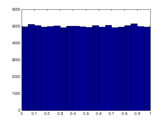
The odds of you winning the last bet are slightly stacked in your favor. There is only a 49% chance your friend wins, but a 51% chance that you win. Lets play the game 100,000 times and see how many times you win, and your friend wins. First, lets generate 100,000 numbers and look at the distribution with a histogram.
N = 100000;
games = rand(N,1);
nbins = 20;
hist(games,nbins)
Now, lets count the number of times you won.
wins = sum(games > 0.49)
losses = sum(games <= 0.49)
sprintf('percent of games won is %1.2f',(wins/N*100))
wins =

       51038


losses =

       48962


ans =

percent of games won is 51.04
random integers uniformly distributed over a range
the rand command gives float numbers between 0 and 1. If you want a random integer, use the randi command.
randi([1 100])
randi([1 100],3,1)
randi([1 100],1,3)
ans =

    65


ans =

    30
    89
    85


ans =

    62     5    97
Normally distributed numbers
The normal distribution is defined by 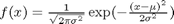 where
where  is the mean value, and
  is the standard deviation. In the standard distribution,
  and
and  .
.
mu = 0; sigma=1;
get a single number
R = mu + sigma*randn
R =

   -0.4563
get a lot of normally distributed numbers
N = 100000;
samples = mu + sigma*randn(N,1);
We define our own bins to do the histogram on
bins = linspace(-5,5);
counts = hist(samples, bins);
Comparing the random distribution to the normal distribution
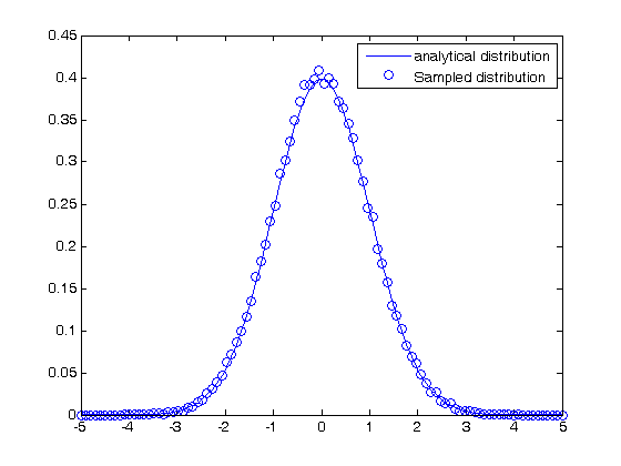
to compare our sampled distribution to the analytical normal distribution, we have to normalize the histogram. The probability density of any bin is defined by the number of counts for that bin divided by the total number of samples divided by the width
the bin width is the range of bins divided by the number of bins.
bin_width = (max(bins)-min(bins))/length(bins);
plot(bins,1/sqrt(2*pi*sigma^2)*exp(-((bins-mu).^2)./(2*sigma^2)),...
bins,counts/N/bin_width,'bo')
legend('analytical distribution','Sampled distribution')
some properties of the normal distribution
What fraction of points lie between plus and minus one standard deviation of the mean?
samples >= mu-sigma will return a vector of ones where the inequality is true, and zeros where it is not. (samples >= mu-sigma) & (samples <= mu+sigma) will return a vector of ones where there is a one in both vectors, and a zero where there is not. In other words, a vector where both inequalities are true. Finally, we can sum the vector to get the number of elements where the two inequalities are true, and finally normalize by the total number of samples to get the fraction of samples that are greater than -sigma and less than sigma.
a1 = sum((samples >= mu-sigma) & (samples <= mu+sigma))/N*100;
sprintf('%1.2f %% of the samples are within plus or minus one standard deviation of the mean.',a1)
ans =

68.44 % of the samples are within plus or minus one standard deviation of the mean.
What fraction of points lie between plus and minus two standard deviations of the mean?
a2 = sum((samples >= mu - 2*sigma) & (samples <= mu + 2*sigma))/N*100;
sprintf('%1.2f %% of the samples are within plus or minus two standard deviations of the mean.',a2)
ans =

95.48 % of the samples are within plus or minus two standard deviations of the mean.
Summary
Matlab has a variety of tools for generating pseudorandom numbers of different types. Keep in mind the numbers are only pseudorandom, but they are still useful for many things as we will see in future posts.
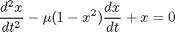
 is a constant. If we let
  http://en.wikipedia.org/wiki/Van_der_Pol_oscillator, then we arrive at this set of equations:
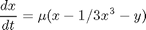

 .
.
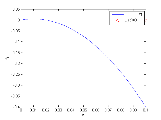
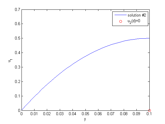
 between two stationary plates separated by distance
  and driven by a pressure drop
  , the governing equations on the velocity
  of the fluid are (assuming flow in the x-direction with the velocity varying only in the y-direction):
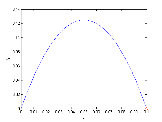
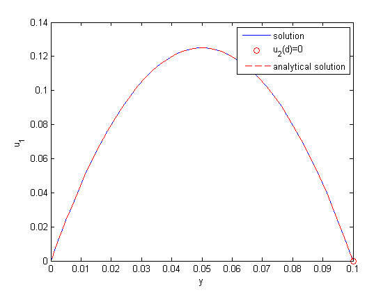
 and
and  , i.e. the no-slip condition at the edges of the plate.
 ,
,  and then
  . This leads to:

 and
and  .
. , and
, and  .
.
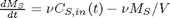 with the initial condition that
 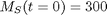 . The wrinkle is that
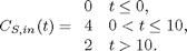
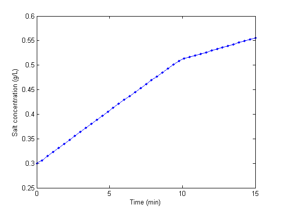 You can see the discontinuity in the salt concentration at 10 minutes due to the discontinous change in the entering salt concentration.
