Conservation of mass in chemical reactions

| categories: uncategorized | View Comments

Conservation of mass in chemical reactions

Conservation of mass in chemical reactions

John Kitchin

Atoms cannot be destroyed in non-nuclear chemical reactions, hence it follows that the same number of atoms entering a reactor must also leave the reactor. The atoms may leave the reactor in a different molecular configuration due to the reaction, but the total mass leaving the reactor must be the same. Here we look at a few ways to show this.

Contents

Water gas shift reaction

We consider the water gas shift reaction : % $CO + H_2O \rightleftharpoons H_2 + CO_2$. We can illustrate the conservation of mass with the following equation: $\bf{\nu}\bf{M}=\bf{0}$. Where $\bf{\nu}$ is the stoichiometric coefficient vector and $\bf{M}$ is a column vector of molecular weights. For simplicity, we use pure isotope molecular weights, and not the isotope-weighted molecular weights.

nu = [-1 -1 1 1];
M = [28; 18; 2; 44];
nu*M
ans =

     0

Atomic mass balances

For any balanced chemical equation, there are the same number of each kind of atom on each side of the equation. Since the mass of each atom is unchanged with reaction, that means the mass of all the species that are reactants must equal the mass of all the species that are products! Here we look at the n C O H

reactants = [-1 -2 -2]
products  = [ 1  2  2]
M = [12.011; 15.999; 1.0079]
reactants =

    -1    -2    -2


products =

     1     2     2


M =

   12.0110
   15.9990
    1.0079

Now if we add the mass of reactants and products, it should sum to zero (since we used the negative sign for stoichiometric coefficients of reactants).

products*M + reactants*M
ans =

     0

Summary

That's all there is to mass conservation with reactions. Nothing changes if there are lots of reactions, as long as each reaction is properly balanced, and none of them are nuclear reactions!

tags: reaction engineering

Read and Post Comments

Interacting with graphs with context menus

| categories: plotting | View Comments

interactive_graph_contextmenu

Contents

Interacting with graphs with context menus

John Kitchin

In Post 1489 we saw how to interact with a contour plot using mouse clicks. That is helpful, but limited to a small number of click types, e.g. left or right clicks, double clicks, etc... And it is not entirely intuitive which one to use if you don't know in advance. In Post 1513 , we increased the functionality by adding key presses to display different pieces of information. While that significantly increases what is possible, it is also difficult to remember what keys to press when there are a lot of them!

Today we examine how to make a context menu that you access by right-clicking on the graph. After you select a menu option, some code is run to do something helpful. We will examine an enthalpy-pressure diagram for steam, and set up functions so you can select one a few thermodynamic functions to display the relevant thermodynamic property under the mouse cursor.

See the video.

function main

The XSteam module makes it pretty easy to generate figures of the steam tables. Here we make the enthalpy-pressure graph.

clear all; close all
P = logspace(-2,3,500); %bar

temps = [1 50 100 150 200 300 400 500 600 700 800]; % degC
figure; hold all
for Ti=temps
    Hh = @(p) XSteam('h_PT',p,Ti);
    H = arrayfun(Hh,P);
    plot(H,P,'k-')
    % add a text label to each isotherm of the temperature
    text(H(end),P(end),sprintf(' %d ^{\\circ}C',Ti),'rotation',90);
end

% add the saturated liquid line
hsat_l = arrayfun(@(p) XSteam('hL_p',p),P);
plot(hsat_l,P)

% add the saturated vapor line
hsat_v = arrayfun(@(p) XSteam('hV_p',p),P);
plot(hsat_v,P)

xlabel('Enthalpy (kJ/kg)')
ylabel('Pressure (bar)')
set(gca,'YScale','log') % this is the traditional view
% adjust axes position so the temperature labels aren't cutoff.
set(gca,'Position',[0.13 0.11 0.775 0.7])

Now we add a textbox to the graph where we will eventually print the thermodynamic properties. We also put a tooltip on the box, which will provide some help if you hold your mouse over it long enough.

textbox_handle = uicontrol('Style','text',...
    'String','Hover mouse here for help',...
     'Position', [0 0 200 25],...
     'TooltipString','Right-click to get a context menu to select a thermodynamic property under the mouse cursor.');

% we will create a simple cursor to show us what point the printed property
% corresponds too
cursor_handle = plot(0,0,'r+');

setup the context menu

hcmenu = uicontextmenu;

Define the context menu items

item1 = uimenu(hcmenu, 'Label', 'H', 'Callback', @hcb1);
item2 = uimenu(hcmenu, 'Label', 'S', 'Callback', @hcb2);
item3 = uimenu(hcmenu, 'Label', 'T', 'Callback', @hcb3);

Now we define the callback functions

    function hcb1(~,~)
        % called when H is selected from the menu
        current_point = get(gca,'Currentpoint');
        H = current_point(1,1);
        P = current_point(1,2);
        set(cursor_handle,'Xdata',H,'Ydata',P)

        % We read H directly from the graph
        str = sprintf('H   = %1.4g kJ/kg', H);
        set(textbox_handle, 'String',str,...
            'FontWeight','bold','FontSize',12)
    end

    function hcb2(~,~)
        % called when S is selected from the menu
        current_point = get(gca,'Currentpoint');
        H = current_point(1,1);
        P = current_point(1,2);
        set(cursor_handle,'Xdata',H,'Ydata',P)

        % To get S, we first need the temperature at the point
        % selected
        T = fzero(@(T) H - XSteam('h_PT',P,T),[1 800]);
        % then we compute the entropy from XSteam
        str = sprintf('S   = %1.4g kJ/kg/K',XSteam('s_PT',P,T));
        set(textbox_handle, 'String',str,...
            'FontWeight','bold','FontSize',12)
    end

    function hcb3(~,~)
        % called when T is selected from the menu
        current_point = get(gca,'Currentpoint');
        H = current_point(1,1);
        P = current_point(1,2);
        set(cursor_handle,'Xdata',H,'Ydata',P)

        % We have to compute the temperature that is consistent with
        % the H,P point selected
        T = fzero(@(T) H - XSteam('h_PT',P,T),[1 800]);
        str = sprintf('T   = %1.4g C',  T);
        set(textbox_handle, 'String',str,...
            'FontWeight','bold','FontSize',12)
    end

set the context menu on the current axes and lines

set(gca,'uicontextmenu',hcmenu)

hlines = findall(gca,'Type','line');
% Attach the context menu to each line
for line = 1:length(hlines)
    set(hlines(line),'uicontextmenu',hcmenu)
end
end

% categories: plotting
% tags: interactive, thermodynamics
Read and Post Comments

Water gas shift equilibria via the NIST Webbook

| categories: miscellaneous, nonlinear algebra | View Comments

Water gas shift equilibria via the NIST Webbook

Water gas shift equilibria via the NIST Webbook

John Kitchin

The NIST webbook provides parameterized models of the enthalpy, entropy and heat capacity of many molecules. In this example, we will examine how to use these to compute the equilibrium constant for the water gas shift reaction $CO + H_2O \rightleftharpoons CO_2 + H_2$ in the temperature range of 500K to 1000K.

Parameters are provided for:

Contents

   Cp = heat capacity (J/mol*K)
   H° = standard enthalpy (kJ/mol)
   S° = standard entropy (J/mol*K)

with models in the form: $Cp^\circ = A + B*t + C*t^2 + D*t^3 +  E/t^2$

$H^\circ - H^\circ_{298.15}= A*t + B*t^2/2 +  C*t^3/3 + D*t^4/4 - E/t + F - H$

$S^\circ = A*ln(t) + B*t + C*t^2/2 + D*t^3/3 -  E/(2*t^2) + G$

where $t=T/1000$, and $T$ is the temperature in Kelvin. We can use this data to calculate equilibrium constants in the following manner. First, we have heats of formation at standard state for each compound; for elements, these are zero by definition, and for non-elements, they have values available from the NIST webbook. There are also values for the absolute entropy at standard state. Then, we have an expression for the change in enthalpy from standard state as defined above, as well as the absolute entropy. From these we can derive the reaction enthalpy, free energy and entropy at standard state, as well as at other temperatures.

We will examine the water gas shift enthalpy, free energy and equilibrium constant from 500K to 1000K, and finally compute the equilibrium composition of a gas feed containing 5 atm of CO and H2 at 1000K.

close all; clear all; clc;

T = linspace(500,1000); % degrees K
t = T/1000;

Setup equations for each species

First we enter in the parameters and compute the enthalpy and entropy for each species.

Hydrogen

link

% T = 298-1000K valid temperature range
A =  33.066178;
B = -11.363417;
C =  11.432816;
D = -2.772874;
E = -0.158558;
F = -9.980797;
G =  172.707974;
H =  0.0;

Hf_29815_H2 = 0.0; % kJ/mol
S_29815_H2 = 130.68; % J/mol/K

dH_H2 = A*t + B*t.^2/2 + C*t.^3/3 + D*t.^4/4 - E./t + F - H;
S_H2 = (A*log(t) + B*t + C*t.^2/2 + D*t.^3/3 - E./(2*t.^2) + G);

H2O

link Note these parameters limit the temperature range we can examine, as these parameters are not valid below 500K. There is another set of parameters for lower temperatures, but we do not consider them here.

% 500-1700 K valid temperature range
A =   30.09200;
B =   6.832514;
C =   6.793435;
D =  -2.534480;
E =   0.082139;
F =  -250.8810;
G =   223.3967;
H =  -241.8264;

Hf_29815_H2O = -241.83; %this is Hf.
S_29815_H2O = 188.84;

dH_H2O = A*t + B*t.^2/2 + C*t.^3/3 + D*t.^4/4 - E./t + F - H;
S_H2O = (A*log(t) + B*t + C*t.^2/2 + D*t.^3/3 - E./(2*t.^2) + G);

CO

link

% 298. - 1300K valid temperature range
A =   25.56759;
B =   6.096130;
C =   4.054656;
D =  -2.671301;
E =   0.131021;
F =  -118.0089;
G =   227.3665;
H = -110.5271;

Hf_29815_CO = -110.53; %this is Hf kJ/mol.
S_29815_CO = 197.66;

dH_CO = A*t + B*t.^2/2 + C*t.^3/3 + D*t.^4/4 - E./t + F - H;
S_CO = (A*log(t) + B*t + C*t.^2/2 + D*t.^3/3 - E./(2*t.^2) + G);

CO2

link

% 298. - 1200.K valid temperature range
A =   24.99735;
B =   55.18696;
C =  -33.69137;
D =   7.948387;
E =  -0.136638;
F =  -403.6075;
G =   228.2431;
H =  -393.5224;

Hf_29815_CO2 = -393.51; %this is Hf.
S_29815_CO2 = 213.79;

dH_CO2 = A*t + B*t.^2/2 + C*t.^3/3 + D*t.^4/4 - E./t + F - H;
S_CO2 = (A*log(t) + B*t + C*t.^2/2 + D*t.^3/3 - E./(2*t.^2) + G);

Standard state heat of reaction

We compute the enthalpy and free energy of reaction at 298.15 K for the following reaction $CO + H2O \rightleftharpoons H2 + CO2$.

Hrxn_29815 = Hf_29815_CO2 + Hf_29815_H2 - Hf_29815_CO - Hf_29815_H2O;
Srxn_29815 = S_29815_CO2 + S_29815_H2 - S_29815_CO - S_29815_H2O;
Grxn_29815 = Hrxn_29815 - 298.15*(Srxn_29815)/1000;

sprintf('deltaH = %1.2f',Hrxn_29815)
sprintf('deltaG = %1.2f',Grxn_29815)
ans =

deltaH = -41.15


ans =

deltaG = -28.62

Correcting $\Delta H$ and $\Delta G$

we have to correct for temperature change away from standard state. We only correct the enthalpy for this temperature change. The correction looks like this:

$$ \Delta H_{rxn}(T) = \Delta H_{rxn}(T_{ref}) + \sum_i \nu_i
(H_i(T)-H_i(T_{ref}))$$

Where $\nu_i$ are the stoichiometric coefficients of each species, with appropriate sign for reactants and products, and $(H_i(T)-H_i(T_{ref})$ is precisely what is calculated for each species with the equations

Hrxn = Hrxn_29815 + dH_CO2 + dH_H2 - dH_CO - dH_H2O;

The entropy is on an absolute scale, so we directly calculate entropy at each temperature. Recall that H is in kJ/mol and S is in J/mol/K, so we divide S by 1000 to make the units match.

Grxn = Hrxn - T.*(S_CO2 + S_H2 - S_CO - S_H2O)/1000;
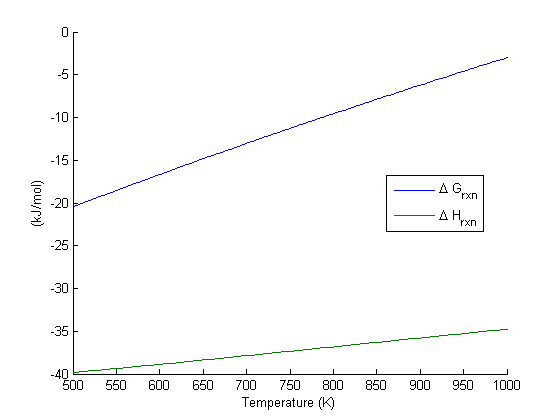
Plot how the $\Delta G$ varies with temperature

over this temperature range the reaction is exothermic, although near 1000K it is just barely exothermic. At higher temperatures we expect the reaction to become endothermic.

figure; hold all
plot(T,Grxn)
plot(T,Hrxn)
xlabel('Temperature (K)')
ylabel('(kJ/mol)')
legend('\Delta G_{rxn}', '\Delta H_{rxn}', 'location','best')

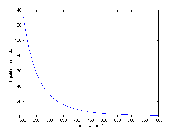
Equilibrium constant calculation

Note the equilibrium constant starts out high, i.e. strongly favoring the formation of products, but drops very quicky with increasing temperature.

R = 8.314e-3; %kJ/mol/K
K = exp(-Grxn/R./T);

figure
plot(T,K)
xlim([500 1000])
xlabel('Temperature (K)')
ylabel('Equilibrium constant')

Equilibrium yield of WGS

Now let's suppose we have a reactor with a feed of H2O and CO at 10atm at 1000K. What is the equilibrium yield of H2? Let $\epsilon$ be the extent of reaction, so that $F_i = F_{i,0} + \nu_i \epsilon$. For reactants, $\nu_i$ is negative, and for products, $\nu_i$ is positive. We have to solve for the extent of reaction that satisfies the equilibrium condition.

A = CO
B = H2O
C = H2
D = CO2
Pa0 = 5; Pb0 = 5; Pc0 = 0; Pd0 = 0;  % pressure in atm
R = 0.082;
Temperature = 1000;

% we can estimate the equilibrium like this. We could also calculate it
% using the equations above, but we would have to evaluate each term. Above
% we simple computed a vector of enthalpies, entropies, etc...
K_Temperature = interp1(T,K,Temperature);

% If we let X be fractional conversion then we have $C_A = C_{A0}(1-X)$,
% $C_B = C_{B0}-C_{A0}X$, $C_C = C_{C0}+C_{A0}X$, and $C_D =
% C_{D0}+C_{A0}X$. We also have $K(T) = (C_C C_D)/(C_A C_B)$, which finally
% reduces to $0 = K(T) - Xeq^2/(1-Xeq)^2$ under these conditions.

f = @(X) K_Temperature - X^2/(1-X)^2;

Xeq = fzero(f,[1e-3 0.999]);
sprintf('The equilibrium conversion for these feed conditions is: %1.2f',Xeq)
ans =

The equilibrium conversion for these feed conditions is: 0.55

Compute gas phase pressures of each species

Since there is no change in moles for this reaction, we can directly calculation the pressures from the equilibrium conversion and the initial pressure of gases. you can see there is a slightly higher pressure of H2 and CO2 than the reactants, consistent with the equilibrium constant of about 1.44 at 1000K. At a lower temperature there would be a much higher yield of the products. For example, at 550K the equilibrium constant is about 58, and the pressure of H2 is 4.4 atm due to a much higher equilibrium conversion of 0.88.

P_CO = Pa0*(1-Xeq)
P_H2O = Pa0*(1-Xeq)
P_H2 = Pa0*Xeq
P_CO2 = Pa0*Xeq
P_CO =

    2.2748


P_H2O =

    2.2748


P_H2 =

    2.7252


P_CO2 =

    2.7252

Compare the equilibrium constants

We can compare the equilibrium constant from the Gibbs free energy and the one from the ratio of pressures. They should be the same!

K_Temperature
(P_CO2*P_H2)/(P_CO*P_H2O)
K_Temperature =

    1.4352


ans =

    1.4352

Summary

The NIST Webbook provides a plethora of data for computing thermodynamic properties. It is a little tedious to enter it all into Matlab, and a little tricky to use the data to estimate temperature dependent reaction energies. A limitation of the Webbook is that it does not tell you have the thermodynamic properties change with pressure. Luckily, those changes tend to be small.

% categories: Miscellaneous, nonlinear algebra
% tags: thermodynamics, reaction engineering
Read and Post Comments

Interacting with graphs with keypresses

| categories: plotting | View Comments

interactive_graph_keypress

Contents

Interacting with graphs with keypresses

John Kitchin

In Post 1489 we saw how to interact with a contour plot using mouse clicks. That is helpful, but limited to a small number of click types, e.g. left or right clicks, double clicks, etc... And it is not entirely intuitive which one to use if you don't know in advance. Today we examine how to make key presses while the mouse is over the graph do something useful. We will examine an enthalpy-pressure diagram for steam, and setup functions so you can press u, s, p, h, or t to display the relevant thermodynamic property under the mouse cursor.

Watch the video here: http://screencast.com/t/nxAiiBXr

function main

The XSteam module makes it pretty easy to generate figures of the steam tables. Here we make the enthalpy-pressure graph.

clear all; close all
P = logspace(-2,3,500); %bar

temps = [1 50 100 150 200 300 400 500 600 700 800]; % degC
figure; hold all
for Ti=temps
    Hh = @(p) XSteam('h_PT',p,Ti);
    H = arrayfun(Hh,P);
    plot(H,P,'k-')
    % add a text label to each isotherm of the temperature
    text(H(end),P(end),sprintf(' %d ^{\\circ}C',Ti),'rotation',90);
end

% add the saturated liquid line
hsat_l = arrayfun(@(p) XSteam('hL_p',p),P);
plot(hsat_l,P)

% add the saturated vapor line
hsat_v = arrayfun(@(p) XSteam('hV_p',p),P);
plot(hsat_v,P)

xlabel('Enthalpy (kJ/kg)')
ylabel('Pressure (bar)')
set(gca,'YScale','log') % this is the traditional view
% adjust axes position so the temperature labels aren't cutoff.
set(gca,'Position',[0.13 0.11 0.775 0.7])

Now we add a textbox to the graph where we will eventually print the thermodynamic properties. We also put a tooltip on the box, which will provide some help if you hold your mouse over it long enough.

textbox_handle = uicontrol('Style','text',...
    'String','',... % start out empty
     'Position', [0 0 200 25],...
     'TooltipString','Press u,s,p,h or t to get the thermodynamic property under the mouse cursor. Ctrl-q to close the figure.');

% we will create a simple cursor to show us what point the printed property
% corresponds too
cursor_handle = plot(0,0,'r+');

Call back functions

we need to define two callback functions that will get called when the mouse moves over the figure, and when a key is pressed.

    function mouse_motion(~,~)
        % since we don't use (gcbo,event) the input arguments, we
        % replace them by ~
        current_point = get(gca,'Currentpoint');
        H = current_point(1,1);
        P = current_point(1,2);
        if (P > 0.01 && P < 1000) && (H > 0.01 && H < 4500)
            set(cursor_handle,'XData',H,'YData',P)
        end
    end

    function keypress_callback(gcbo,event)
        % We get the point under the cursor.
        H = get(cursor_handle,'XData');
        P = get(cursor_handle,'YData');

        % solve  for T
        T = fzero(@(T) H - XSteam('h_PT',P,T),[1 800]);

        % now define a string for each type of key press.
        str = ''; % default string to display
        switch event.Key
            case 'u'
                % compute internal energy for the P,T under cursor
                str = sprintf('U   = %1.4g kJ/kg', XSteam('u_PT',P,T));
            case 's'
                % compute entropy for the P,T under cursor
                str = sprintf('S   = %1.4g kJ/kg/K',XSteam('s_PT',P,T));
            case 'p'
                str = sprintf('P   = %1.4g bar',P);
            case 'h'
                str = sprintf('H   = %1.4g kJ/kg', H);
            case 't'
                str = sprintf('T   = %1.4g C',  T);
            case 'uparrow'
                if strcmp(event.Modifier,'control')
                    set(cursor_handle,'YData', P + 10)
                else
                    set(cursor_handle,'YData', P + 100)
                end
            case 'downarrow'
                if strcmp(event.Modifier,'control')
                    set(cursor_handle,'YData', P - 10)
                else
                    set(cursor_handle,'YData', P - 100)
                end
            case 'leftarrow'
                if strcmp(event.Modifier,'control')
                    set(cursor_handle,'XData', H - 10)
                else
                    set(cursor_handle,'XData', H - 100)
                end
            case 'rightarrow'
                if strcmp(event.Modifier,'control')
                    set(cursor_handle,'XData', H + 10)
                else
                    set(cursor_handle,'XData', H + 100)
                end
            case 'q'
                % quit. We use a dialog box to make sure we really
                % want to quit, in case q was accidentally pressed.
                choice = questdlg('Are you sure you want to quit?','','yes','no','no');
                switch choice
                    case 'yes'
                        close
                        return
                    case 'no'
                        str = '';
                end
            otherwise
                str = '';
        end

        % and put the string in our text box
        set(textbox_handle, 'String',str,...
            'FontWeight','bold','FontSize',12)
    end

finally, attach the callback functions to the current figure.

set(gcf,'KeyPressFcn',@keypress_callback)
set(gcf,'WindowButtonMotionFcn',@mouse_motion)
end

% categories: plotting
% tags: interactive, thermodynamics
% post_id = 1513; %delete this line to force new post;
% permaLink = http://matlab.cheme.cmu.edu/2011/12/07/interacting-with-graphs-with-keypresses/;
Read and Post Comments

Turkeyfy your plots

| categories: plotting | View Comments

turkeyfy

Contents

Turkeyfy your plots

John Kitchin

Need to make a festive graph? Today we look at putting a background graphic in your plot.

close all; clear all

Boring plot for thanksgiving

After a plateful of turkey you won't be able to keep your eyes open looking at this graph!

x = linspace(0,400,10);
y = x.^2;
plot(x,y)
title('Happy Thanksgiving')
xlabel('x')
ylabel('y')

Spice it up!

Let's add a background image, use a festive plot color, and a festive font.

Read the figure in

[X,MAP] = imread('8happy-thanksgiving-day.gif');

Plot the figure

note we have to flip it over so it comes out right,and set the colormap. the image is scaled by the xy data we have above. The image will be upside down for now, and the y-axis will be going in the wrong direction. we will fix that later.

image([min(x) max(x)], [min(y) max(y)], flipud(X));
colormap(MAP)

Plot data over the image

Hint: use the listfonts command to see what fonts are available on your machine.

hold on
plot(x,y,'o-','color',cmu.colors('Crimson glory'),'linewidth',2,...
    'markerfacecolor',cmu.colors('Crimson glory'))

title('Happy Thanksgiving','FontName','Lucida Handwriting')
xlabel('x','FontName','Lucida Handwriting')
ylabel('y','FontName','Lucida Handwriting')

Finally fix the y-axis

this makes the graph look like what you want! Much more festive.

set(gca,'ydir','normal');

% categories: plotting
% tags: whimsical
Read and Post Comments

« Previous Page -- Next Page »