Better interpolate than never

| categories: basic matlab | View Comments

interp_methods

Contents

Better interpolate than never

John Kitchin

close all; clear all

We often have some data that we have obtained in the lab, and we want to solve some problem using the data. For example, suppose we have this data that describes the value of f at time t.

t = [0.5 1 3 6]
f = [0.6065    0.3679    0.0498    0.0025]
plot(t,f)
xlabel('t')
ylabel('f(t)')
t =

    0.5000    1.0000    3.0000    6.0000


f =

    0.6065    0.3679    0.0498    0.0025

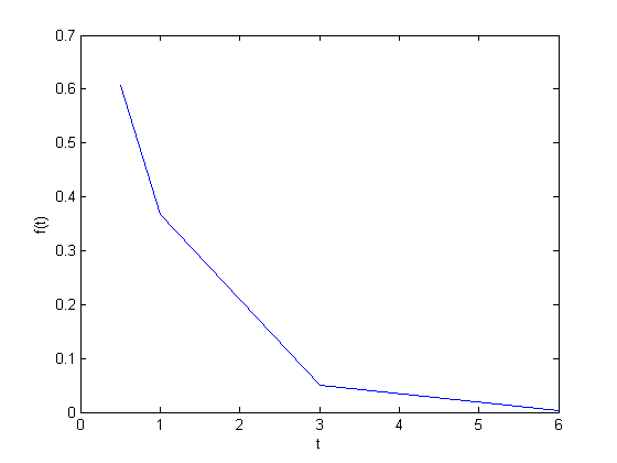
Estimate the value of f at t=2.

This is a simple interpolation problem.

interp1(t,f,2)
ans =

    0.2089

The function we sample above is actually f(t) = exp(-t). The linearly interpolated example isn't too accurate.

exp(-2)
ans =

    0.1353

improved interpolation

we can tell Matlab to use a better interpolation scheme: cubic polynomial splines like this. For this example, it only slightly improves the interpolated answer. That is because you are trying to estimate the value of an exponential function with a cubic polynomial, it fits better than a line, but it can't accurately reproduce the exponential function.

interp1(t,f,2,'cubic')
ans =

    0.1502

The inverse question

It is easy to interpolate a new value of f given a value of t. What if we want to know the time that f=0.2? We can approach this a few ways.

method 1

we setup an equation that interpolates f for us. Then, we setup another function that we can use fsolve on. The second function will be equal to zero at the time. The second function will look like 0 = 6.25 - f(t). The answer for 0.2=exp(-t) is t = 1.6094. Since we use interpolation here, we will get an approximate answer. The first method is not to bad.

func = @(time) interp1(t,f,time);
g = @(time) 0.2 - func(time);

initial_guess = 2;
ans = fsolve(g, initial_guess)
Equation solved.

fsolve completed because the vector of function values is near zero
as measured by the default value of the function tolerance, and
the problem appears regular as measured by the gradient.


ans =

    2.0556

method 2: switch the interpolation order

We can switch the order of the interpolation to solve this problem.

interp1(f,t,0.2)
interp1(f,t,0.2,'cubic')
ans =

    2.0556


ans =

    1.5980

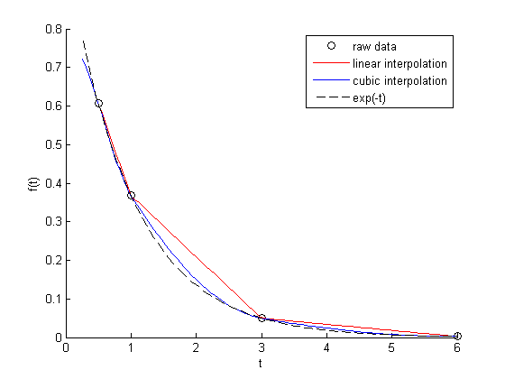
Note we get the same answer with linear interpolation, but a different answer with the cubic interpolation. Here the cubic interpolation does much better job of fitting. You can see why in this figure. The cubic interpolation is much closer to the true function over most of the range. Although, note that it overestimates in some regions and underestimates in other regions.

figure
hold all
x = linspace(0.25, 6);
plot(t,f,'ko ')
plot(x, interp1(t,f,x),'r-')
plot(x, interp1(t,f,x,'cubic'),'b-')
plot(x,exp(-x),'k--')
xlabel('t')
ylabel('f(t)')
legend('raw data','linear interpolation','cubic interpolation','exp(-t)')

A harder problem

Suppose we want to know at what time is 1/f = 100? Now we have to decide what do we interpolate: f(t) or 1/f(t). Let's look at both ways and decide what is best. The answer to $1/exp(-t) = 100$ is 4.6052

interpolate on f(t) then invert the interpolated number

g2 = @(time) 100 - 1./func(time);
initial_guess = 4.5;
a1 = fsolve(g2, initial_guess)
sprintf('%%error = %1.2f',((a1 - 4.6052)/2.5*100))
Equation solved.

fsolve completed because the vector of function values is near zero
as measured by the default value of the function tolerance, and
the problem appears regular as measured by the gradient.


a1 =

    5.5243


ans =

%error = 36.76

invert f(t) then interpolate on 1/f

ifunc2 = @(time) interp1(t,1./f,time);
g5 = @(time) 100 - ifunc2(time);
a2 = fsolve(g5, initial_guess)
sprintf('%%error = %1.2f',((a2 - 4.6052)/2.5*100))
Equation solved.

fsolve completed because the vector of function values is near zero
as measured by the default value of the function tolerance, and
the problem appears regular as measured by the gradient.


a2 =

    3.6311


ans =

%error = -38.96

discussion

In this case you get different errors, one overestimates and one underestimates the answer, and by a lot: ~plus or minus 37% . Let's look at what is happening.

plotting 1/f

figure
hold all
x = linspace(0.25, 6);
plot(t,1./f,'ko ')
plot(x, 1./interp1(t,f,x),'r-')
plot(x, interp1(t,1./f,x,'cubic'),'b-')
plot(x,1./exp(-x),'k--')
xlabel('t')
ylabel('1/f(t)')
legend('raw data','linear interpolation','cubic interpolation','1/exp(-t)')

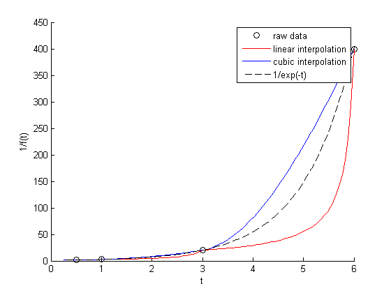
You can see that the cubic interpolation is overestimating the true function between 3 and 6, while the linear interpolation underestimates it. This is an example of where you clearly need more data in that range to make good estimates. Neither interpolation method is doing a great job. The trouble in reality is that you often do not know the real function to do this analysis. Here you can say the time is probably between 3.6 and 5.5 where 1/f(t) = 100, but you can't read much more than that into it. If you need a more precise answer, you need better data, or you need to use an approach other than interpolation. For example, you could fit an exponential function to the data and use that to estimate values at other times.

'done'

% categories: basic matlab
% tags: interpolation
ans =

done

Read and Post Comments

are two averages different?

| categories: data analysis | View Comments

are two averages different?

are two averages different?

John Kitchin 1/28/2012

adapted from http://stattrek.com/ap-statistics-4/unpaired-means.aspx

Contents

Class A had 30 students who received an average test score of 78, with standard deviation of 10. Class B had 25 students an average test score of 85, with a standard deviation of 15. We want to know if the difference in these averages is statistically relevant. Note that we only have estimates of the true average and standard deviation for each class, and there is uncertainty in those estimates. As a result, we are unsure if the averages are really different. It could have just been luck that a few students in class B did better.

The hypothesis:

the true averages are the same. We need to perform a two-sample t-test of the hypothesis that $\mu_1 - \mu_2 = 0$ (this is often called the null hypothesis). we use a two-tailed test because we do not care if the difference is positive or negative, either way means the averages are not the same.

the data

n1 = 30; % students in class A
x1 = 78; % average grade in class A
s1 = 10; % std dev of exam grade in class A

n2 = 25; % students in class B
x2 = 85; % average grade in class B
s2 = 15; % std dev of exam grade in class B

Compute the standard error

this is the standard error of the difference between the two averages. Note the standard error of the difference is less than the standard error of the individual averages.

SE = sqrt(s1^2/n1 + s2^2/n2)
SE =

    3.5119

calculate degrees of freedom

see the discussion at http://stattrek.com/Help/Glossary.aspx?Target=Two-sample%20t-test for a more complex definition of degrees of freedom. Here we simply subtract one from each sample size to account for the estimation of the average of each sample.

DF = (n1 - 1) + (n2 - 1)
DF =

    53

compute the t-score for our data

The difference between two averages determined from small sample numbers follows the t-distribution. the t-score is the difference between the difference of the means and the hypothesized difference of the means, normalized by the standard error. we compute the absolute value of the t-score to make sure it is positive for convenience later.

tscore = abs(((x1 - x2)-0)/SE)
tscore =

    1.9932

Interpretation

A way to approach determinining if the difference is significant or not is to ask, does our computed average fall within a confidence range of the hypothesized value (zero)? If it does, then we can attribute the difference to statistical variations at that confidence level. If it does not, we can say that statistical variations do not account for the difference at that confidence level, and hence the averages must be different.

Lets compute the t-value that corresponds to a 95% confidence level for a mean of zero with the degrees of freedom computed earlier. This means that 95% of the t-scores we expect to get will fall within $\pm$ t95.

ci = 0.95;
alpha = 1 - ci;
t95 = tinv(1-alpha/2, DF)
t95 =

    2.0057

since tscore < t95, we conclude that at the 95% confidence level we cannot say these averages are statistically different because our computed t-score falls in the expected range of deviations. Note that our t-score is very close to the 95% limit. Let's consider a smaller confidence interval.

ci = 0.94;
alpha = 1 - ci;
t94 = tinv(1-alpha/2, DF)
t94 =

    1.9219

at the 94% confidence level, however, tscore > t94, which means we can say with 94% confidence that the two averages are different; class B performed better than class A did. Alternatively, there is only about a 6% chance we are wrong about that statement.

another way to get there

An alternative way to get the confidence that the averages are different is to directly compute it from the cumulative t-distribution function. We compute the difference between all the t-values less than tscore and the t-values less than -tscore, which is the fraction of measurements that are between them. You can see here that we are practically 95% sure that the averages are different.

f = tcdf(tscore,DF)-tcdf(-tscore,DF)
f =

    0.9486

'done'
% categories: data analysis
ans =

done

Read and Post Comments

Sums, products and linear algebra notation - avoiding loops where possible

| categories: linear algebra | View Comments

Sums, products and linear algebra notation - avoiding loops where possible

Sums, products and linear algebra notation - avoiding loops where possible

John Kitchin

Today we examine some methods of linear algebra that allow us to avoid writing explicit loops in Matlab for some kinds of mathematical operations.

Contents

Consider the operation on two vectors $\bf{a}$ and $\bf{b}$.

$$y=\sum\limits_{i=1}^n a_ib_i$$

a = [1 2 3 4 5];
b = [3 6 8 9 10];

Old-fashioned way with a loop

We can compute this with a loop, where you initialize y, and then add the product of the ith elements of a and b to y in each iteration of the loop. This is known to be slow for large vectors

y = 0;
for i=1:length(a)
    y = y + a(i)*b(i);
end

y
y =

   125

dot notation

Matlab defines dot operators, so we can compute the element-wise product of $\bf{a}$ and $\bf{b}$, and then use the builtin sum command to get the result.

y = sum(a.*b)
y =

   125

dot product

The operation above is formally the definition of a dot product. We can directly compute this in Matlab. Note that one vector must be transposed so that we have the right dimensions for legal matrix multiplication (one vector must be a row, and one must be column). It does not matter which order the multiplication is done as shown here.

y = a*b'

y = b*a'
y =

   125


y =

   125

Another example

$$y=\sum\limits_{i=1}^n w_ix_i^2$$

This operation is like a weighted sum of squares.

w = [0.1 0.25 0.12 0.45 0.98];
x = [9 7 11 12 8];

Old-fashioned method with a loop

y = 0;
for i = 1:length(w)
    y = y + w(i)*x(i)^2;
end
y
y =

  162.3900

dot operator approach

We use parentheses to ensure that x is squared element-wise before the element-wise multiplication.

y = sum(w.*(x.^2))
y =

  162.3900

Linear algebra approach

The operation is mathematically equivalent to $y = \bf{x}\bf{D_w}\bf{x^T}$ when $\bf{x}$ is a row vector. $\bf{D_w}$ is a diagonal matrix with the values of $\bf{w}$ on the diagonal, and zeros everywhere else. The Matlab command diag creates this matrix conveniently.

y = x*diag(w)*x'
y =

  162.3900

Last example

$$z=\sum\limits_{i=1}^n w_i x_i y_i$$

This operation is like a weighted sum of products.

w = [0.1 0.25 0.12 0.45 0.98];
x = [9 7 11 12 8];
y = [2 5 3 8 0];

Old fashioned method with a loop

z = 0;
for i=1:length(w)
    z = z + w(i)*x(i)*y(i);
end
z
z =

   57.7100

dot notation

we use parentheses

z = sum(w.*x.*y)
z =

   57.7100

Linear algebra approach

Note that it does not matter what order the dot products are done in, just as it does not matter what order w(i)*x(i)*y(i) is multiplied in.

z = x*diag(w)*y'
z = y*diag(x)*w'
z = w*diag(y)*x'
z =

   57.7100


z =

   57.7100


z =

   57.7100

Summary

We showed examples of the following equalities between traditional sum notations and linear algebra

$$\bf{a}\bf{b}=\sum\limits_{i=1}^n a_ib_i$$

$$\bf{x}\bf{D_w}\bf{x^T}=\sum\limits_{i=1}^n w_ix_i^2$$

$$\bf{x}\bf{D_w}\bf{y^T}=\sum\limits_{i=1}^n w_i x_i y_i$$

These relationships enable one to write the sums as a single line of Matlab code, which utilizes fast linear algebra subroutines, avoids the construction of slow loops, and reduces the opportunity for errors in the code. Admittedly, it introduces the opportunity for new types of errors, like using the wrong relationship, or linear algebra errors due to matrix size mismatches.

% categories: Linear Algebra
% tags: math
Read and Post Comments

Estimating the boiling point of water

| categories: uncategorized | View Comments

water_boilingpoint

Contents

Estimating the boiling point of water

John Kitchin

I got distracted looking for Shomate parameters for ethane today, and came across this website on predicting the boiling point of water using the Shomate equations. The basic idea is to find the temperature where the Gibbs energy of water as a vapor is equal to the Gibbs energy of the liquid.

clear all; close all

Liquid water

http://webbook.nist.gov/cgi/cbook.cgi?ID=C7732185&Units=SI&Mask=2#Thermo-Condensed valid over 298-500

Hf_liq = -285.830; % kJ/mol
S_liq = 0.06995;   % kJ/mol/K
shomateL = [-203.6060
            1523.290
           -3196.413
            2474.455
               3.855326
            -256.5478
            -488.7163
            -285.8304];

Gas phase water

http://webbook.nist.gov/cgi/cbook.cgi?ID=C7732185&Units=SI&Mask=1&Type=JANAFG&Table=on#JANAFG

Interestingly, these parameters are listed as valid only above 500K. That means we have to extrapolate the values down to 298K. That is risky for polynomial models, as they can deviate substantially outside the region they were fitted to.

Hf_gas = -241.826; % kJ/mol
S_gas = 0.188835;  % kJ/mol/K

shomateG = [30.09200
             6.832514
             6.793435
            -2.534480
             0.082139
          -250.8810
           223.3967
          -241.8264];

Compute G over a range of temperatures.

T = linspace(0,200)' + 273.15; % temperature range from 0 to 200 degC

t = T/1000;

% normalize sTT by 1/1000  so entropies are in kJ/mol/K
sTT = [log(t) t t.^2/2 t.^3/3 -1./(2*t.^2) 0*t.^0 t.^0 0*t.^0]/1000;
hTT = [t t.^2/2 t.^3/3 t.^4/4 -1./t 1*t.^0 0*t.^0 -1*t.^0];

Gliq = Hf_liq + hTT*shomateL - T.*(sTT*shomateL);
Ggas = Hf_gas + hTT*shomateG - T.*(sTT*shomateG);

Interpolate the difference between the two vectors to find the boiling point

The boiling point is where Gliq = Ggas, so we solve Gliq(T)-Ggas(T)=0 to find the point where the two free energies are equal.

f = @(t) interp1(T,Gliq-Ggas,t);
bp = fzero(f,373)
bp =

  373.2045

Plot the two free energies

You can see the intersection occurs at approximately 100 degC.

plot(T-273.15,Gliq,T-273.15,Ggas)
line([bp bp]-273.15,[min(Gliq) max(Gliq)])
legend('liquid water','steam')
xlabel('Temperature \circC')
ylabel('\DeltaG (kJ/mol)')
title(sprintf('The boiling point is approximately %1.2f \\circC', bp-273.15))

Summary

The answer we get us 0.05 K too high, which is not bad considering we estimated it using parameters that were fitted to thermodynamic data and that had finite precision and extrapolated the steam properties below the region the parameters were stated to be valid for.

% tags: thermodynamics
Read and Post Comments

Gibbs energy minimization and the NIST webbook

| categories: optimization | View Comments

Gibbs energy minimization and the NIST webbook

Gibbs energy minimization and the NIST webbook

John Kitchin

Contents

In Post 1536 we used the NIST webbook to compute a temperature dependent Gibbs energy of reaction, and then used a reaction extent variable to compute the equilibrium concentrations of each species for the water gas shift reaction.

Today, we look at the direct minimization of the Gibbs free energy of the species, with no assumptions about stoichiometry of reactions. We only apply the constraint of conservation of atoms. We use the NIST Webbook to provide the data for the Gibbs energy of each species.

As a reminder we consider equilibrium between the species $CO$, $H_2O$, $CO_2$ and $H_2$, at 1000K, and 10 atm total pressure with an initial equimolar molar flow rate of $CO$ and $H_2O$.

Links to data

H2

H2O

CO

CO2

function nist_wb_constrained_min
T = 1000; %K
R = 8.314e-3; % kJ/mol/K

P = 10; % atm, this is the total pressure in the reactor
Po = 1; % atm, this is the standard state pressure

We define species like this.

We are going to store all the data and calculations in vectors, so we need to assign each position in the vector to a species. Here are the definitions we use in this work.

1  CO
2  H2O
3  CO2
4  H2
species = {'CO' 'H2O' 'CO2' 'H2'};

Heats of formation at 298.15 K

Hf298 = [
    -110.53  % CO
    -241.826 % H2O
    -393.51  % CO2
       0.0]; % H2

Shomate parameters for each species

   A             B           C          D          E       F          G       H
WB = [25.56759  6.096130     4.054656  -2.671301  0.131021 -118.0089 227.3665   -110.5271  % CO
      30.09200  6.832514     6.793435  -2.534480  0.082139 -250.8810 223.3967   -241.8264    % H2O
      24.99735  55.18696   -33.69137    7.948387 -0.136638 -403.6075 228.2431   -393.5224   % CO2
      33.066178 -11.363417  11.432816  -2.772874 -0.158558 -9.980797 172.707974    0.0]; % H2

Shomate equations

t = T/1000;
T_H = [t; t^2/2; t^3/3; t^4/4; -1/t; 1; 0; -1];
T_S = [log(t); t; t^2/2; t^3/3; -1/(2*t^2); 0; 1; 0];

H = WB*T_H; % (H - H_298.15) kJ/mol
S = WB*T_S/1000; % absolute entropy kJ/mol/K

Gjo = Hf298 + H - T*S; % Gibbs energy of each component at 1000 K

Gibbs energy of mixture

this function assumes the ideal gas law for the activities

    function G = func(nj)
        Enj = sum(nj);
        G = sum(nj.*(Gjo'/R/T + log(nj/Enj*P/Po)));
    end

Elemental conservation constraints

We impose the constraint that all atoms are conserved from the initial conditions to the equilibrium distribution of species. These constraints are in the form of A_eq x = beq, where x is the vector of mole numbers. CO H2O CO2 H2

Aeq = [ 1    0    1    0   % C balance
        1    1    2    0   % O balance
        0    2    0    2]; % H balance

% equimolar feed of 1 mol H2O and 1 mol CO
beq = [1   % mol C fed
       2   % mol O fed
       2]; % mol H fed

Constraints on bounds

This simply ensures there are no negative mole numbers.

LB = [0 0 0];

Solve the minimization problem

x0 = [0.5 0.5 0.5 0.5]; % initial guesses

options = optimset('Algorithm','sqp');
x = fmincon(@func,x0,[],[],Aeq,beq,LB,[],[],options)
Local minimum found that satisfies the constraints.

Optimization completed because the objective function is non-decreasing in 
feasible directions, to within the default value of the function tolerance,
and constraints are satisfied to within the default value of the constraint tolerance.


x =

    0.4549    0.4549    0.5451    0.5451

Compute mole fractions and partial pressures

The pressures here are in good agreement with the pressures found in Post 1536 . The minor disagreement (in the third or fourth decimal place) is likely due to convergence tolerances in the different algorithms used.

yj = x/sum(x);
Pj = yj*P;

for i=1:numel(x)
    fprintf('%5d%10s%15.4f atm\n',i, species{i}, Pj(i))
end
    1        CO         2.2745 atm
    2       H2O         2.2745 atm
    3       CO2         2.7255 atm
    4        H2         2.7255 atm

Computing equilibrium constants

We can compute the equilibrium constant for the reaction $CO + H_2O \rightleftharpoons CO_2 + H_2$. Compared to the value of K = 1.44 we found at the end of Post 1536 , the agreement is excellent. Note, that to define an equilibrium constant it is necessary to specify a reaction, even though it is not necessary to even consider a reaction to obtain the equilibrium distribution of species!

nuj = [-1 -1 1 1]; % stoichiometric coefficients of the reaction
K = prod(yj.^nuj)
K =

    1.4359

end

% categories: optimization
% tags: Thermodynamics, reaction engineering
Read and Post Comments

« Previous Page -- Next Page »