Matlab in Chemical Engineering at CMU

Contents

Better interpolate than never

John Kitchin

close all; clear all

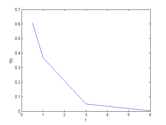
We often have some data that we have obtained in the lab, and we want to solve some problem using the data. For example, suppose we have this data that describes the value of f at time t.

t = [0.5 1 3 6]
f = [0.6065    0.3679    0.0498    0.0025]
plot(t,f)
xlabel('t')
ylabel('f(t)')

t =

    0.5000    1.0000    3.0000    6.0000


f =

    0.6065    0.3679    0.0498    0.0025

Estimate the value of f at t=2.

This is a simple interpolation problem.

interp1(t,f,2)

ans =

    0.2089

The function we sample above is actually f(t) = exp(-t). The linearly interpolated example isn't too accurate.

exp(-2)

ans =

    0.1353

improved interpolation

we can tell Matlab to use a better interpolation scheme: cubic polynomial splines like this. For this example, it only slightly improves the interpolated answer. That is because you are trying to estimate the value of an exponential function with a cubic polynomial, it fits better than a line, but it can't accurately reproduce the exponential function.

interp1(t,f,2,'cubic')

ans =

    0.1502

The inverse question

It is easy to interpolate a new value of f given a value of t. What if we want to know the time that f=0.2? We can approach this a few ways.

method 1

we setup an equation that interpolates f for us. Then, we setup another function that we can use fsolve on. The second function will be equal to zero at the time. The second function will look like 0 = 6.25 - f(t). The answer for 0.2=exp(-t) is t = 1.6094. Since we use interpolation here, we will get an approximate answer. The first method is not to bad.

func = @(time) interp1(t,f,time);
g = @(time) 0.2 - func(time);

initial_guess = 2;
ans = fsolve(g, initial_guess)

Equation solved.

fsolve completed because the vector of function values is near zero
as measured by the default value of the function tolerance, and
the problem appears regular as measured by the gradient.




ans =

    2.0556

method 2: switch the interpolation order

We can switch the order of the interpolation to solve this problem.

interp1(f,t,0.2)
interp1(f,t,0.2,'cubic')

ans =

    2.0556


ans =

    1.5980

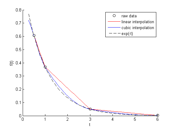
Note we get the same answer with linear interpolation, but a different answer with the cubic interpolation. Here the cubic interpolation does much better job of fitting. You can see why in this figure. The cubic interpolation is much closer to the true function over most of the range. Although, note that it overestimates in some regions and underestimates in other regions.

figure
hold all
x = linspace(0.25, 6);
plot(t,f,'ko ')
plot(x, interp1(t,f,x),'r-')
plot(x, interp1(t,f,x,'cubic'),'b-')
plot(x,exp(-x),'k--')
xlabel('t')
ylabel('f(t)')
legend('raw data','linear interpolation','cubic interpolation','exp(-t)')

A harder problem

Suppose we want to know at what time is 1/f = 100? Now we have to decide what do we interpolate: f(t) or 1/f(t). Let's look at both ways and decide what is best. The answer to is 4.6052

interpolate on f(t) then invert the interpolated number

g2 = @(time) 100 - 1./func(time);
initial_guess = 4.5;
a1 = fsolve(g2, initial_guess)
sprintf('%%error = %1.2f',((a1 - 4.6052)/2.5*100))

Equation solved.

fsolve completed because the vector of function values is near zero
as measured by the default value of the function tolerance, and
the problem appears regular as measured by the gradient.




a1 =

    5.5243


ans =

%error = 36.76

invert f(t) then interpolate on 1/f

ifunc2 = @(time) interp1(t,1./f,time);
g5 = @(time) 100 - ifunc2(time);
a2 = fsolve(g5, initial_guess)
sprintf('%%error = %1.2f',((a2 - 4.6052)/2.5*100))

Equation solved.

fsolve completed because the vector of function values is near zero
as measured by the default value of the function tolerance, and
the problem appears regular as measured by the gradient.




a2 =

    3.6311


ans =

%error = -38.96

discussion

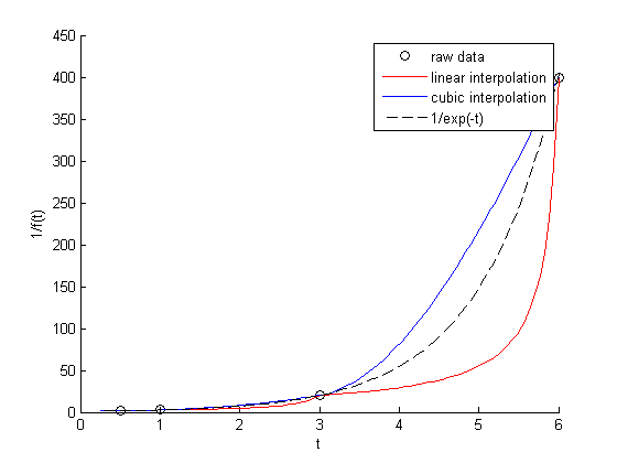
In this case you get different errors, one overestimates and one underestimates the answer, and by a lot: ~plus or minus 37% . Let's look at what is happening.

plotting 1/f

figure
hold all
x = linspace(0.25, 6);
plot(t,1./f,'ko ')
plot(x, 1./interp1(t,f,x),'r-')
plot(x, interp1(t,1./f,x,'cubic'),'b-')
plot(x,1./exp(-x),'k--')
xlabel('t')
ylabel('1/f(t)')
legend('raw data','linear interpolation','cubic interpolation','1/exp(-t)')

You can see that the cubic interpolation is overestimating the true function between 3 and 6, while the linear interpolation underestimates it. This is an example of where you clearly need more data in that range to make good estimates. Neither interpolation method is doing a great job. The trouble in reality is that you often do not know the real function to do this analysis. Here you can say the time is probably between 3.6 and 5.5 where 1/f(t) = 100, but you can't read much more than that into it. If you need a more precise answer, you need better data, or you need to use an approach other than interpolation. For example, you could fit an exponential function to the data and use that to estimate values at other times.

'done'

% categories: basic matlab
% tags: interpolation

ans =

done

Published with MATLAB® 7.13