Linear algebra approaches to solving systems of constant coefficient ODEs

| categories: linear algebra, odes | View Comments

const_coeff_coupled

Contents

Linear algebra approaches to solving systems of constant coefficient ODEs

John Kitchin

Today we consider how to solve a system of first order, constant coefficient ordinary differential equations using linear algebra. These equations could be solved numerically, but in this case there are analytical solutions that can be derived. The equations we will solve are:

$y'_1 = -0.02 y_1 + 0.02 y_2$

$y'_2 = 0.02 y_1 - 0.02 y_2$

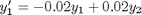
We can express this set of equations in matrix form as: $\left[\begin{array}{c}y'_1\\y'_2\end{array}\right] = \left[\begin{array}{cc} -0.02 & 0.02 \\ 0.02 & -0.02\end{array}\right] \left[\begin{array}{c}y_1\\y_2\end{array}\right]$

The general solution to this set of equations is

$\left[\begin{array}{c}y_1\\y_2\end{array}\right] = \left[\begin{array}{cc}v_1 & v_2\end{array}\right] \left[\begin{array}{cc} c_1 & 0 \\ 0 & c_2\end{array}\right] \exp\left(\left[\begin{array}{cc} \lambda_1 & 0 \\ 0 & \lambda_2\end{array}\right] \left[\begin{array}{c}t\\t\end{array}\right]\right)$

where $\left[\begin{array}{cc} \lambda_1 & 0 \\ 0 & \lambda_2\end{array}\right]$ is a diagonal matrix of the eigenvalues of the constant coefficient matrix, $\left[\begin{array}{cc}v_1 & v_2\end{array}\right]$ is a matrix of eigenvectors where the $i^{th}$ column corresponds to the eigenvector of the $i^{th}$ eigenvalue, and $\left[\begin{array}{cc} c_1 & 0 \\ 0 & c_2\end{array}\right]$ is a matrix determined by the initial conditions.

In this example, we evaluate the solution using linear algebra. The initial conditions we will consider are $y_1(0)=0$ and $y_2(0)=150$.

close all
A = [-0.02 0.02;
    0.02 -0.02];

get the eigenvalues and eigenvectors of the A matrix

[V,D] = eig(A)
V =

    0.7071    0.7071
   -0.7071    0.7071


D =

   -0.0400         0
         0         0

V is a matrix of the eigenvectors, with each column being an eigenvector. Note that the eigenvectors are normalized so their length equals one. D is a diagonal matrix of eigenvalues.

Compute the $c$ matrix

V*c = Y0

We can solve this equation easily with the \ operator. As written, c will be a vector, but we need it in the form of a diagonal matrix, so we wrap the solution in the diag command.

Y0 = [0; 150]; % initial conditions
c = diag(V\Y0)
c =

 -106.0660         0
         0  106.0660

Constructing the solution

We will create a vector of time values, and stack them for each solution, $y_1(t)$ and $Y_2(t)$.

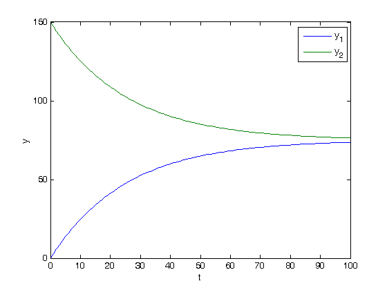
t = linspace(0,100);
T = [t;t];

y = V*c*exp(D*T);
plot(t,y)
xlabel('t')
ylabel('y')
legend 'y_1' 'y_2'

Verifying the solution

One way we can verify the solution is to analytically compute the derivatives from the differential equations, and then compare those derivatives to numerically evaluated derivatives from the solutions.

yp = A*y; % analytical derivatives

% numerically evaluated derivatves
yp1 = cmu.der.derc(t,y(1,:));
yp2 = cmu.der.derc(t,y(2,:));

plot(t,yp,t,yp1,'g--',t,yp2,'r--')
legend 'y''_1 analytical' 'y''_2 analytical' 'y''_1 numerical' 'y''_2 numerical'
xlabel('t')
ylabel('dy/dt')

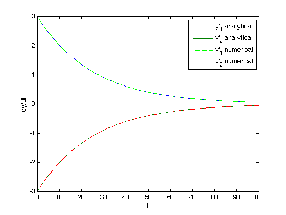
What you can see here is that the analytical derivatives are visually equivalent to the numerical derivatives of the solution we derived.

'done'
% categories: ODEs, linear algebra
% tags: math
ans =

done

Read and Post Comments

The trapezoidal method of integration

| categories: basic matlab | View Comments

trapezoidal_integration

Contents

The trapezoidal method of integration

John Kitchin

See http://en.wikipedia.org/wiki/Trapezoidal_rule

$$\int_a^b f(x) dx \approx \frac{1}{2}\displaystyle\sum\limits_{k=1}^N(x_{k+1}-x_k)(f(x_{k+1}) + f(x_k))$$

Let's compute the integral of sin(x) from x=0 to $\pi$
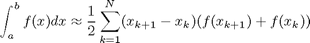
. To approximate the integral, we need to divide the interval from $a$ to $b$ into $N$ intervals. The analytical answer is 2.0.

We will use this example to illustrate the difference in performance between loops and vectorized operations in Matlab.

a = 0; b = pi;
N = 1000; % this is the number of intervals

h = (b - a)/N; % this is the width of each interval
x = a:h:b; % note there are N+1 elements in this x vector
y = sin(x); % the sin function is already vectorized, so y contains N+1 elements

Trapezoid method using a loop

we use the tic and toc functions to time how long it takes to run.

tic
f = 0;
for k=1:N
    f = f + 0.5*((x(k+1)-x(k))*(y(k+1)+y(k)));
end
f
toc
f =

    2.0000

Elapsed time is 0.002520 seconds.

vectorized approach

tic
Xk = x(2:end)-x(1:end-1); % vectorized version of (x(k+1)-x(k))
Yk = y(2:end)+y(1:end-1); % vectorized version of (y(k+1)+y(k))

f = 0.5*sum(Xk.*Yk) % vectorized version of the loop above
toc

% It isn't strictly necessary to calculate Xk this way, since here by
% design every interval is the same width, but this approach would work for
% non-uniform x-values.
f =

    2.0000

Elapsed time is 0.000148 seconds.

total linear algebra way

In the last example, there may be loop buried in the sum command. Lets do one final method, using linear algebra, in a single line. The key to understanding this is to recognize the sum is just the result of a dot product of the x differences and y sums. We have to transpose the y sums to get the vector dimensions to work for the dot product (* is matrix multiplication/dot product in Matlab

tic
f = 0.5*(x(2:end)-x(1:end-1))*(y(2:end)+y(1:end-1))'
toc
f =

    2.0000

Elapsed time is 0.000130 seconds.

summary

The loop method is straightforward to code, and looks alot like the formula that defines the trapezoid method. the vectorized methods are not as easy to read, and take fewer lines of code to write. However, the vectorized methods are much faster than the loop, so the loss of readability could be worth it for very large problems.

% categories: basic matlab
% tags: math

% post_id = 1231; %delete this line to force new post;
% permaLink = http://matlab.cheme.cmu.edu/2011/10/14/the-trapezoidal-method-of-integration/;
Read and Post Comments

nonlinearfit_minsse.m

| categories: data analysis | View Comments

nonlinearfit_minsse

Contents

function main
% y = x^a
close all; clear all; clc
x = [0 1.1 2.3 3.1 4.05 6];
y = [0.0039    1.2270    5.7035   10.6472   18.6032   42.3024];

Plot the raw data

the data appears to be polynomial or exponential. In this case, a must be greater than 1, since the data is clearly not linear.

plot(x,y,'ko ')
xlabel('x')
ylabel('y')

getting an initial guess

The best a will minimize the summed squared error between the model and the fit. At the end, we define two nested functions: one is the model function that gives the predicted y-values from an arbitrary a parameter, and the x data, and the second computes the summed squared error between the model and data for a value of a. Here we plot the summed squared error function as a function of a.

arange = linspace(1,3,20);
sse = arrayfun(@errfunc,arange);

plot(arange,sse)
xlabel('a')
ylabel('\Sigma (y-y_{pred})^2')

Minimization of the summed squared error

based on the graph above, you can see a minimum in the summed squared error near a = 2.1. We use that as our initial guess

pars = fminsearch(@errfunc,2.1)

figure; hold all
plot(x,y,'bo ')
plot(x,model(pars,x))
xlabel('x')
ylabel('y')
legend('data','fit')
pars =

    2.0901

summary

We can do nonlinear fitting by directly minimizing the summed squared error between a model and data. This method lacks some of the features of nlinfit, notably the simple ability to get the confidence interval. However, this method is more flexible and powerful than nlinfit, and may work in times where nlinfit fails.

nested functions

    function yp = model(pars,X)
        a = pars(1);
        yp = X.^a; % predicted values
    end

    function sse = errfunc(pars)
        % calculates summed squared error
        pred_y = model(pars,x);
        err = pred_y - y;
        sse = sum(err.^2);
    end
end

% categories: data analysis
Read and Post Comments

Graphical methods to help get initial guesses for multivariate nonlinear regression

| categories: data analysis, plotting | View Comments

Graphical methods to help get initial guesses for multivariate nonlinear regression

Graphical methods to help get initial guesses for multivariate nonlinear regression

John Kitchin

Contents

Goal

fit the model f(x1,x2; a,b) = a*x1 + x2^b to the data given below. This model has two independent variables, and two paramters.

function main
close all

given data

Note it is not easy to visualize this data in 2D, but we can see the function in 3D.

x1 = [1 2 3 4 5 6]';
x2 = [.2 .4 .8 .9 1.1 2.1]';
X = [x1 x2]; % independent variables

f = [ 3.3079    6.6358   10.3143   13.6492   17.2755   23.6271]';

plot3(x1,x2,f)
xlabel('x1')
ylabel('x2')
zlabel('f(x1,x2)')

Strategy

we want to do a nonlinear fit to find a and b that minimize the summed squared errors between the model predictions and the data. With only two variables, we can graph how the summed squared error varies with the parameters, which may help us get initial guesses . Let's assume the parameters lie in a range, here we choose 0 to 5. In other problems you would adjust this as needed.

arange = linspace(0,5);
brange = linspace(0,5);

Create arrays of all the possible parameter values

[A,B] = meshgrid(arange, brange);

now evaluate SSE(a,b)

we use the arrayfun to evaluate the error function for every pair of a,b from the A,B matrices

SSE = arrayfun(@errfunc,A,B);

plot the SSE data

we use a contour plot because it is easy to see where minima are. Here the colorbar shows us that dark blue is where the minimum values of the contours are. We can see the minimum is near a=3.2, and b = 2.1 by using the data exploration tools in the graph window.

contourf(A,B,SSE,50)
colorbar
xlabel('a')
ylabel('b')

hold on
plot(3.2, 2.1, 'ro')
text(3.4,2.2,'Minimum near here','color','r')

Now the nonlinear fit with our guesses

guesses = [3.18,2.02];
[pars residuals J] = nlinfit(X,f,@model, guesses)
parci = nlparci(pars,residuals,'jacobian',J,'alpha',0.05)

% show where the best fit is on the contour plot.
plot(pars(1),pars(2),'r*')
text(pars(1)+0.1,pars(2),'Actual minimum','color','r')
pars =

    3.2169    1.9728


residuals =

    0.0492
    0.0379
    0.0196
   -0.0309
   -0.0161
    0.0034


J =

    1.0000   -0.0673
    2.0000   -0.1503
    3.0000   -0.1437
    4.0000   -0.0856
    5.0000    0.1150
    6.0000    3.2067


parci =

    3.2034    3.2305
    1.9326    2.0130

Compare the fit to the data in a plot

figure
hold all
plot3(x1,x2,f,'ko ')
plot3(x1,x2,model(pars,[x1 x2]),'r-')
xlabel('x1')
ylabel('x2')
zlabel('f(x1,x2)')
legend('data','fit')
view(-12,20) % adjust viewing angle to see the curve better.

Summary

It can be difficult to figure out initial guesses for nonlinear fitting problems. For one and two dimensional systems, graphical techniques may be useful to visualize how the summed squared error between the model and data depends on the parameters.

Nested function definitions

    function f = model(pars,X)
        % Nested function for the model
        x1 = X(:,1);
        x2 = X(:,2);
        a = pars(1);
        b = pars(2);
        f = a*x1 + x2.^b;
    end

    function sse = errfunc(a,b)
        % Nested function for the summed squared error
        fit = model([a b],X);
        sse = sum((fit - f).^2);
    end
end

% categories: data analysis, plotting
Read and Post Comments

Sprintfing to the finish

| categories: basic matlab | View Comments

sprintfing

Contents

Sprintfing to the finish

John Kitchin

There are many times where you need to control the format of how variables are displayed in Matlab. A crude way to control this is through the format command. By default, Matlab shows decimal numbers on a fixed scale with 5 decimals.

1/3
0.25
10.1
ans =

    0.3333


ans =

    0.2500


ans =

   10.1000

To show more decimals, you can issue a 'format long' command

format long
1/3
0.25
10.1

% to reset the format to the default, simply call format
format
ans =

   0.333333333333333


ans =

   0.250000000000000


ans =

  10.100000000000000

But suppose you want to print results with the correct number of significant figures, which will vary. For that, you need the sprintf command. The sprintf command takes a string, with a format specifier in it, and replaces the format specifier with a numeric value. A typical specifier for a decimal number is %w.df, where w is the width of the field, and d is the number of decimals, or precision. The field width is the minimum number of characters to print. See the documentation for sprintf (doc sprintf) for much more detail. To print with only two decimal places, consider these two examples

n = 1/3;
a = sprintf('%1.2f', n)
a =

0.33

You can embed the format strings into a string

a = sprintf('The value of 1/3 to two decimal places is %1.2f', n)
% Note that sprintf returns a string, that can be used in other
% places.
a =

The value of 1/3 to two decimal places is 0.33

You can have more than one format string in a string, and then you have to have more than one value to pass to each format string. The values get passed in order.

sprintf('value 1 = %1.2f and value 2 = %1.4f', 1/3,1/6)
ans =

value 1 = 0.33 and value 2 = 0.1667

You can reuse a format string several times for multiple values

sprintf('The answers are: %1.2f  ', [1/3 1/6 1/9])
ans =

The answers are: 0.33  The answers are: 0.17  The answers are: 0.11  

Note that the whole string is repeated for each element in the array. To get a better output, we might put a carriage return after each line like this

sprintf('The answers are: %1.2f\n', [1/3 1/6 1/9])
ans =

The answers are: 0.33
The answers are: 0.17
The answers are: 0.11


Significant digit specification

If you know how many significant digits you want, we use the %g format string. To get 1/3 to 3 significant digits:

sprintf('%1.3g',1/3)
% Note the first zero is not significant
sprintf('%1.3g',4/3)
% Note we know this to lower precision, because the first digit is
% significant.
ans =

0.333


ans =

1.33

modifier flags to format strings

If you want to print a +- sign with the data, compare these two outputs:

sprintf('%1.2f\n',[-1 1])
% the decimals do not align, making it a little harder to read
ans =

-1.00
1.00


sprintf('%+1.2f\n',[-1 1])
% here the decimals align, and it is easier to read.
ans =

-1.00
+1.00


Scientific notation

the eps command gives you the smallest possible spacing between float numbers in matlab.

eps
ans =

  2.2204e-016

As a float, this number is practically zero to many decimal places. As a decimal, it is impractical to view.

sprintf('%1.12f',eps)
ans =

0.000000000000

Instead, we use scientific notation

a = sprintf('%1.2e',eps)
a =

2.22e-016

you can combine the string output with this syntax.

['the answer is: '  a]
ans =

the answer is: 2.22e-016

Or you can use fprintf

fprintf('the answer is: %1.2e\n',eps)
% What is the difference between fprintf and sprintf? fprintf prints
% directly to the screen, and does not output any result, avoiding the
the answer is: 2.22e-016
ans = ....
in the display window. So if you don't need the string output as a
variable, the results are cleaner with sprintf.

Summary

That is how simple it is to control the format of how your data is displayed. There are more options than shown here, but this is the majority of formatting I find necessary most of the time.

'done'

% categories: basic matlab
ans =

done

Read and Post Comments

« Previous Page -- Next Page »