Matlab in Chemical Engineering at CMU

Contents

function main

% y = x^a
close all; clear all; clc
x = [0 1.1 2.3 3.1 4.05 6];
y = [0.0039    1.2270    5.7035   10.6472   18.6032   42.3024];

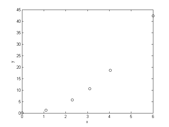
Plot the raw data

the data appears to be polynomial or exponential. In this case, a must be greater than 1, since the data is clearly not linear.

plot(x,y,'ko ')
xlabel('x')
ylabel('y')

getting an initial guess

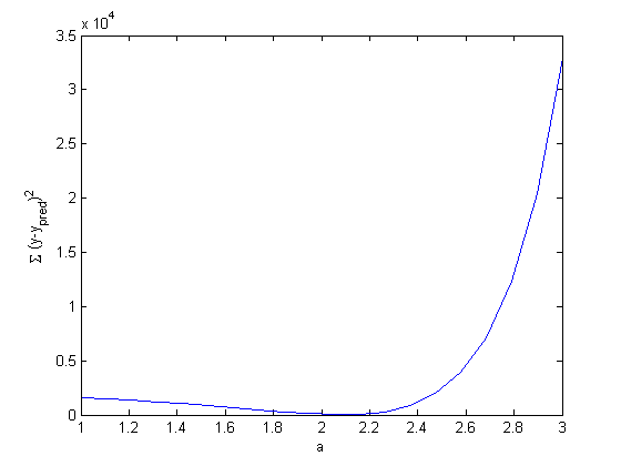
The best a will minimize the summed squared error between the model and the fit. At the end, we define two nested functions: one is the model function that gives the predicted y-values from an arbitrary a parameter, and the x data, and the second computes the summed squared error between the model and data for a value of a. Here we plot the summed squared error function as a function of a.

arange = linspace(1,3,20);
sse = arrayfun(@errfunc,arange);

plot(arange,sse)
xlabel('a')
ylabel('\Sigma (y-y_{pred})^2')

Minimization of the summed squared error

based on the graph above, you can see a minimum in the summed squared error near a = 2.1. We use that as our initial guess

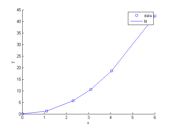
pars = fminsearch(@errfunc,2.1)

figure; hold all
plot(x,y,'bo ')
plot(x,model(pars,x))
xlabel('x')
ylabel('y')
legend('data','fit')

pars =

    2.0901

summary

We can do nonlinear fitting by directly minimizing the summed squared error between a model and data. This method lacks some of the features of nlinfit, notably the simple ability to get the confidence interval. However, this method is more flexible and powerful than nlinfit, and may work in times where nlinfit fails.

nested functions

    function yp = model(pars,X)
        a = pars(1);
        yp = X.^a; % predicted values
    end

    function sse = errfunc(pars)
        % calculates summed squared error
        pred_y = model(pars,x);
        err = pred_y - y;
        sse = sum(err.^2);
    end

end

% categories: data analysis

Published with MATLAB® 7.13