Linear algebra approaches to solving systems of constant coefficient ODEs
October 21, 2011 at 12:46 AM | categories: linear algebra, odes | View Comments
Contents
Linear algebra approaches to solving systems of constant coefficient ODEs
John Kitchin
Today we consider how to solve a system of first order, constant coefficient ordinary differential equations using linear algebra. These equations could be solved numerically, but in this case there are analytical solutions that can be derived. The equations we will solve are:


We can express this set of equations in matrix form as: ![$\left[\begin{array}{c}y'_1\\y'_2\end{array}\right] = \left[\begin{array}{cc} -0.02 & 0.02 \\ 0.02 & -0.02\end{array}\right] \left[\begin{array}{c}y_1\\y_2\end{array}\right]$](http://matlab.cheme.cmu.edu/wp-content/uploads/2011/10/const_coeff_coupled_eq84697.png)
The general solution to this set of equations is
![$\left[\begin{array}{c}y_1\\y_2\end{array}\right] = \left[\begin{array}{cc}v_1 & v_2\end{array}\right] \left[\begin{array}{cc} c_1 & 0 \\ 0 & c_2\end{array}\right] \exp\left(\left[\begin{array}{cc} \lambda_1 & 0 \\ 0 & \lambda_2\end{array}\right] \left[\begin{array}{c}t\\t\end{array}\right]\right)$](http://matlab.cheme.cmu.edu/wp-content/uploads/2011/10/const_coeff_coupled_eq32208.png)
where ![$\left[\begin{array}{cc} \lambda_1 & 0 \\ 0 & \lambda_2\end{array}\right]$](http://matlab.cheme.cmu.edu/wp-content/uploads/2011/10/const_coeff_coupled_eq06652.png) is a diagonal matrix of the eigenvalues of the constant coefficient matrix,
is a diagonal matrix of the eigenvalues of the constant coefficient matrix, ![$\left[\begin{array}{cc}v_1 & v_2\end{array}\right]$](http://matlab.cheme.cmu.edu/wp-content/uploads/2011/10/const_coeff_coupled_eq51102.png) is a matrix of eigenvectors where the
is a matrix of eigenvectors where the  column corresponds to the eigenvector of the
  eigenvalue, and
 ![$\left[\begin{array}{cc} c_1 & 0 \\ 0 & c_2\end{array}\right]$](http://matlab.cheme.cmu.edu/wp-content/uploads/2011/10/const_coeff_coupled_eq84783.png) is a matrix determined by the initial conditions.
is a matrix determined by the initial conditions.
In this example, we evaluate the solution using linear algebra. The initial conditions we will consider are  and
and  .
.
close all
A = [-0.02 0.02;
    0.02 -0.02];
get the eigenvalues and eigenvectors of the A matrix
[V,D] = eig(A)
V =

    0.7071    0.7071
   -0.7071    0.7071


D =

   -0.0400         0
         0         0
V is a matrix of the eigenvectors, with each column being an eigenvector. Note that the eigenvectors are normalized so their length equals one. D is a diagonal matrix of eigenvalues.
Compute the  matrix
V*c = Y0
We can solve this equation easily with the \ operator. As written, c will be a vector, but we need it in the form of a diagonal matrix, so we wrap the solution in the diag command.
Y0 = [0; 150]; % initial conditions
c = diag(V\Y0)
c =

 -106.0660         0
         0  106.0660
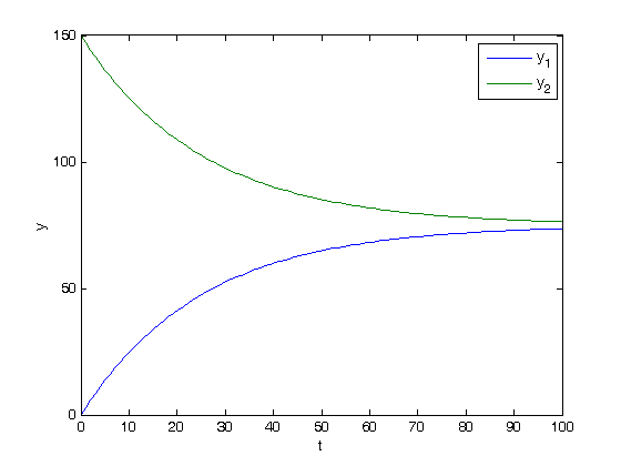
Constructing the solution
We will create a vector of time values, and stack them for each solution,  and
and  .
.
t = linspace(0,100);
T = [t;t];

y = V*c*exp(D*T);
plot(t,y)
xlabel('t')
ylabel('y')
legend 'y_1' 'y_2'

Verifying the solution
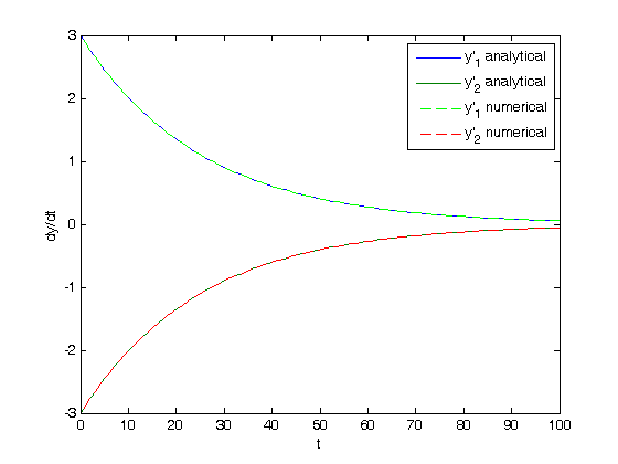
One way we can verify the solution is to analytically compute the derivatives from the differential equations, and then compare those derivatives to numerically evaluated derivatives from the solutions.
yp = A*y; % analytical derivatives

% numerically evaluated derivatves
yp1 = cmu.der.derc(t,y(1,:));
yp2 = cmu.der.derc(t,y(2,:));

plot(t,yp,t,yp1,'g--',t,yp2,'r--')
legend 'y''_1 analytical' 'y''_2 analytical' 'y''_1 numerical' 'y''_2 numerical'
xlabel('t')
ylabel('dy/dt')

What you can see here is that the analytical derivatives are visually equivalent to the numerical derivatives of the solution we derived.
'done'
% categories: ODEs, linear algebra
% tags: math
ans =

done
 matrix