Counting roots

September 10, 2011 at 11:06 PM | categories: odes, nonlinear algebra | View Comments

Counting roots

John Kitchin

Problem statement
Use roots for this polynomial
Plot the function to see where the roots are
method 1
method 1a
Discussion
Method 2

Problem statement

The goal here is to determine how many roots there are in a nonlinear function we are interested in solving. For this example, we use a cubic polynomial because we know there are three roots.

$$f(x) = x^3 + 6x^2 - 4x -24$$

function main

clc; clear all; close all;

Use roots for this polynomial

This ony works for a polynomial, it does not work for any other nonlinear function.

roots([1 6 -4 -24])

ans =

   -6.0000
    2.0000
   -2.0000

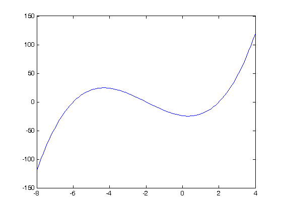
Plot the function to see where the roots are

x = linspace(-8,4);
fx = x.^3 + 6*x.^2 - 4*x - 24;
plot(x,fx)

method 1

count the number of times the sign changes in the interval. We determine the sign of each element (-1, 0 or +1) and then use a a loop to go through each element. A sign change is detected when an element is not equal to the previous element. Note this is not foolproof; we may over count roots if we get a sequence -1 0 1. We check for that by making sure neither of the two elements being compared are zero.

sign_fx = sign(fx);

count = 0;
for i=2:length(sign_fx)
    if sign_fx(i) ~= sign_fx(i-1) && sign_fx(i) ~= 0 && sign_fx(i-1) ~= 0
        count = count + 1;
        disp(sprintf('A root is between x = %f and %f',x(i-1),x(i)))
    end
end

disp(sprintf('The number of sign changes is %i.',count))

A root is between x = -6.060606 and -5.939394
A root is between x = -2.060606 and -1.939394
A root is between x = 1.939394 and 2.060606
The number of sign changes is 3.

method 1a

this one line code also counts sign changes. the diff command makes all adjacent, identical elements equal zero, and sign changes = 2 (1 - (-1)) or (-1 - 1). Then we just sum up the diff vector, divide by two, and that is the number of roots. Note that no check for 0 is needed; you will get 1/2 a sign change from -1 to 0. and another half from 0 to 1. They add up to a whole sign change.

sum(abs(diff(sign_fx))/2)

ans =

     3

Discussion

Method 1 is functional but requires some programming. Method 1a is concise but probably tricky to remember.

Method 2

using events in an ODE solver Matlab can identify events in the solution to an ODE, for example, when a function has a certain value, e.g. f(x) = 0. We can take advantage of this to find the roots and number of roots in this case.

$$f'(x) = 3x^2 + 12x - 4$$

with f(-8) = -120

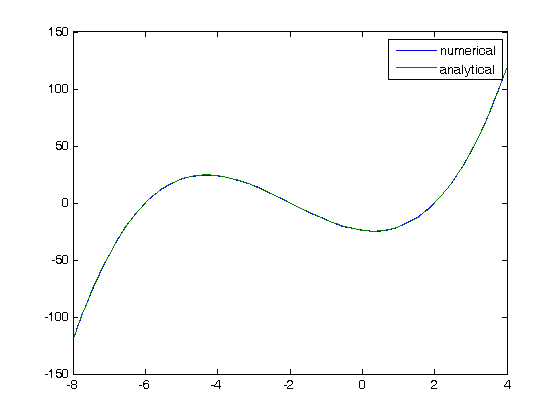
xspan = [-8 4];
fp0 = -120;

options = odeset('Events',@event_function);
[X,Y,XE,VE,IE] = ode45(@myode,xspan,fp0,options);
XE % these are the x-values where the function equals zero
nroots = length(XE);
disp(sprintf('Found %i roots in the x interval',nroots))

% lets compare the solution to the  original function to make sure they are
% the same.
figure
plot(X,Y,x,fx)
legend 'numerical' 'analytical'

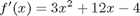
function dfdx = myode(x,f)
dfdx = 3*x^2 + 12*x - 4;

function [value,isterminal,direction] = event_function(t,y)
value = y - 0;  % then value = 0, an event is triggered
isterminal = 0; % do not terminate after the first event
direction = 0;  % get all the zeros

% categories: ODEs, nonlinear algebra

XE =

   -6.0000
   -2.0000
    2.0000

Found 3 roots in the x interval

Read and Post Comments

Plane Poiseuille flow - BVP solve by shooting method

September 08, 2011 at 06:24 PM | categories: odes | View Comments

Plane Poiseuille flow - BVP solve by shooting method

In Post 878 learned how to use the BVP solver in Matlab to solve a boundary value problem. Another approach is to use the shooting method. The reason we can't use an initial value solver for a BVP is that there is not enough information at the initial value to start. In the shooting method, we take the function value at the initial point, and guess what the function derivatives are so that we can do an integration. If our guess was good, then the solution will go through the known second boundary point. If not, we guess again, until we get the answer we need. In this example we repeat the pressure driven flow example, but illustrate the shooting method.

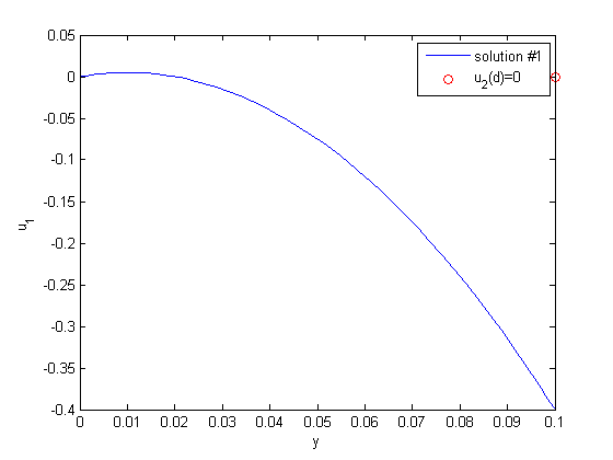
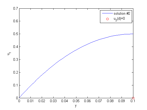
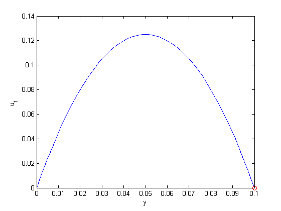
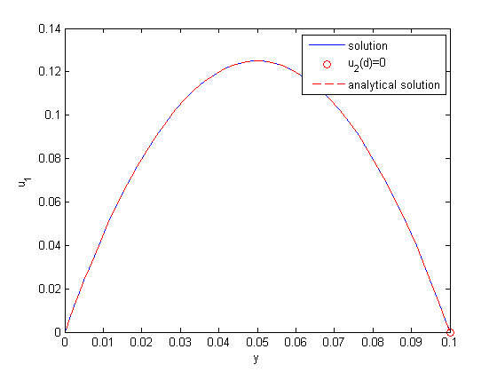
In the pressure driven flow of a fluid with viscosity $\mu$ between two stationary plates separated by distance $d$ and driven by a pressure drop $\Delta P/\Delta x$ , the governing equations on the velocity $u$ of the fluid are (assuming flow in the x-direction with the velocity varying only in the y-direction):

First guess
second guess
Using a solver
Plot final solution
Known analytical solution

$\frac{\Delta P}{\Delta x} = \mu \frac{d^2u}{dy^2}$

with boundary conditions $u(y=0) = 0$ and $u(y=d) = 0$ , i.e. the no-slip condition at the edges of the plate.

we convert this second order BVP to a system of ODEs by letting $u_1 = u$ , $u_2 = u_1'$ and then $u_2' = u_1''$ . This leads to:

$\frac{d u_1}{dy} = u_2$

$\frac{d u_2}{dy} = \frac{1}{\mu}\frac{\Delta P}{\Delta x}$

with boundary conditions $u_1(y=0) = 0$ and $u_1(y=d) = 0$ .

for this problem we let the plate separation be d=0.1, the viscosity $\mu = 1$ , and $\frac{\Delta P}{\Delta x} = -100$ .

function main

clc; close all; clear all;

d = 0.1; % plate thickness

First guess

we need u_1(0) and u_2(0), but we only have u_1(0). We need to guess a value for u_2(0) and see if the solution goes through the u_2(d)=0 boundary value.

u1_0 = 0; % known
u2_0 = 1; % guessed

init = [u1_0 u2_0];
dspan = [0 d];
[y,U] = ode45(@odefun,dspan,init);
plot(y,U(:,1),[d],[0],'ro')
legend 'solution #1' 'u_2(d)=0'
xlabel('y')
ylabel('u_1')
% It appears we have undershot, so our initial slope was not large
% enough

second guess

u1_0 = 0; % known
u2_0 = 10; % guessed

init = [u1_0 u2_0];
dspan = [0 d];
[y,U] = ode45(@odefun,dspan,init);
plot(y,U(:,1),[d],[0],'ro')
legend 'solution #2' 'u_2(d)=0'
xlabel('y')
ylabel('u_1')
% Now we have overshot, the initial slope is too high. The right
% answer must be between 1 and 10 You could continue to iterate on
% this manually until the value of u_1(d) = 0. Instead, we use a
% solver to do that, now that we have a reasonable guess for u_2(0).

Using a solver

we have to make a function that is equal to zero when u_2(d) = 0.

u2_guess = 2;
u2_0_solved = fsolve(@myfunc,u2_guess)

Equation solved.

fsolve completed because the vector of function values is near zero
as measured by the default value of the function tolerance, and
the problem appears regular as measured by the gradient.




u2_0_solved =

    5.0000

Plot final solution

init = [u1_0 u2_0_solved];
dspan = [0 d];
[y,U] = ode45(@odefun,dspan,init);

figure
plot(y,U(:,1),d,0,'ro')
xlabel('y')
ylabel('u_1')

Known analytical solution

the analytical solution to this problem is known, and we can plot it on top of the numerical solution

mu = 1;
Pdrop = -100; % this is DeltaP/Deltax
u = -(Pdrop)*d^2/2/mu*(y/d-(y/d).^2);
hold all
plot(y,u,'r--')
legend 'solution' 'u_2(d)=0' 'analytical solution'

'done'

ans =

done

Finally, the solutions agree, and show that the velocity profile is parabolic, with a maximum in the middle of the two plates. You can also see that the velocity at each boundary is zero, as required by the boundary conditions

function dUdy = odefun(y,U)
% here we define our differential equations
u1 = U(1);
u2 = U(2);

mu = 1;
Pdrop = -100; % this is DeltaP/Deltax
du1dy = u2;
du2dy = 1/mu*Pdrop;
dUdy = [du1dy; du2dy];


function Z = myfunc(u2_guess)
% this function is zero when u_1(d) = 0.
u1_0 = 0; % known
u2_0 = u2_guess; % guessed
d = 0.1;

init = [u1_0 u2_0];
dspan = [0 d];
sol = ode45(@odefun,dspan,init);

u = deval(sol,d); % u = [u_1(d) u_2(d)]
u1_d = u(1);
Z = u1_d;

% categories: ODEs
% tags: math, fluids, bvp


% post_id = 1036; %delete this line to force new post;

Read and Post Comments

Stopping the integration of an ODE at some condition

September 02, 2011 at 03:27 PM | categories: odes | View Comments

Stopping the integration of an ODE at some condition

John Kitchin

In Post 968 we learned how to get the numerical solution to an ODE, and then to use the deval function to solve the solution for a particular value. The deval function uses interpolation to evaluate the solution at other valuse. An alternative approach would be to stop the ODE integration when the solution has the value you want. That can be done in Matlab by using an "event". You setup an event function and tell the ode solver to use it by setting an option.

The problem

The problem

given that the concentration of a species A in a constant volume, batch reactor obeys this differential equation $\frac{dC_A}{dt}=- k C_A^2$ with the initial condition $C_A(t=0) = 2.3$ mol/L and $k = 0.23$ L/mol/s, compute the time it takes for $C_A$ to be reduced to 1 mol/L.

function main

clear all; close all; clc

k = 0.23;
Cao = 2.3;
tspan = [0 10];

% create an options variable
options = odeset('Events',@event_function);

% note the extra outputs
[t,Ca,TE,VE] = ode45(@myode,tspan,Cao,options);

TE % this is the time value where the event occurred
VE % this is the value of Ca where the event occurred

sprintf('At t = %1.2f seconds the concentration of A is %1.2f mol/L.', TE,VE)

TE =

    2.4598


VE =

    1.0000


ans =

At t = 2.46 seconds the concentration of A is 1.00 mol/L.

plot(t,Ca)
xlabel('Time (sec)')
ylabel('C_A (mol/L)')
% you can see the integration terminated at Ca = 1

'done'

ans =

done

function dCadt = myode(t,Ca)
k = 0.23;
dCadt = -k*Ca^2;

function [value,isterminal,direction] = event_function(t,Ca)

% when value is equal to zero, an event is triggered.
% set isterminal to 1 to stop the solver at the first event, or 0 to
% get all the events.
%  direction=0 if all zeros are to be computed (the default), +1 if
%  only zeros where the event function is increasing, and -1 if only
%  zeros where the event function is decreasing.
value = Ca - 1.0;  % when value = 0, an event is triggered
isterminal = 1; % terminate after the first event
direction = 0;  % get all the zeros

% categories: ODEs
% tags: reaction engineering

Read and Post Comments

ODEs with discontinuous forcing functions

September 01, 2011 at 01:56 PM | categories: odes | View Comments

ODEs with discontinuous forcing functions

John Kitchin

Problem statement
Solution

Problem statement

Adapted from http://archives.math.utk.edu/ICTCM/VOL18/S046/paper.pdf A mixing tank initially contains 300 g of salt mixed into 1000 L of water. at t=0 min, a solution of 4 g/L salt enters the tank at 6 L/min. at t=10 min, the solution is changed to 2 g/L salt, still entering at 6 L/min. The tank is well stirred, and the tank solution leaves at a rate of 6 L/min. Plot the concentration of salt (g/L) in the tank as a function of time.

Solution

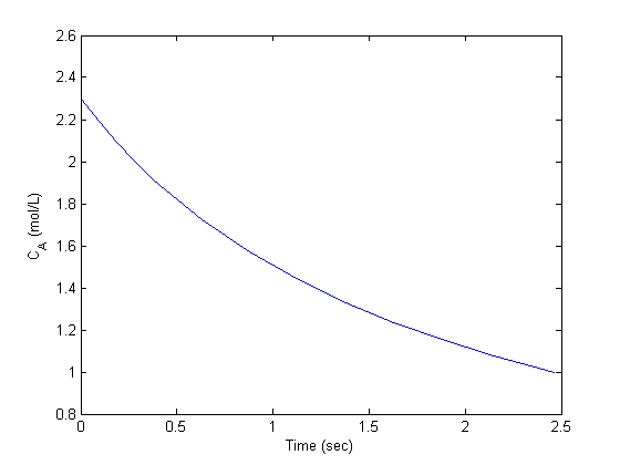
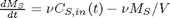
A mass balance on the salt in the tank leads to this differential equation: $\frac{dM_S}{dt} = \nu C_{S,in}(t) - \nu M_S/V$ with the initial condition that $M_S(t=0)=300$

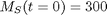
. The wrinkle is that $C_{S,in}(t) = \begin{array}{ll}�0 & t \le 0, \\�4 & 0 < t \le 10, \\�2 & t > 10. \end{array}$

function main

tspan = [0,15]; % min
Mo = 300; % gm salt
[t,M] = ode45(@mass_balance,tspan,Mo);

V = 1000; % L
plot(t,M/V,'b.-')
xlabel('Time (min)')
ylabel('Salt concentration (g/L)')

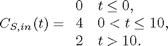
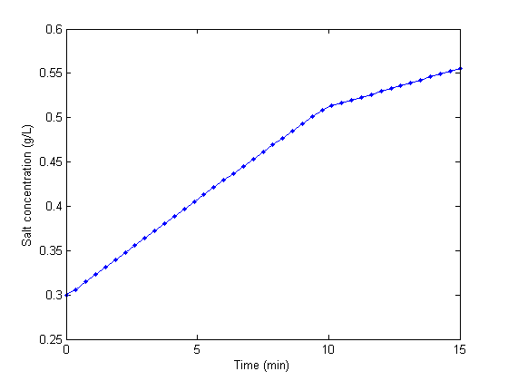
You can see the discontinuity in the salt concentration at 10 minutes due to the discontinous change in the entering salt concentration.

'done'

ans =

done

discontinuous feed concentration function

function Cs = Cs_in(t)

if t < 0
    Cs = 0; % g/L
elseif t > 0 && t <= 10
    Cs = 4; % g/L
else
    Cs = 2; % g/L
end

$\frac{dM_S}{dt} = \nu C_{S,in}(t) - \nu M_S/V$

function dMsdt = mass_balance(t,Ms)

V = 1000; % L
nu = 6;   % L/min
dMsdt = nu*Cs_in(t) - nu*Ms/V;

% categories: ODEs

Read and Post Comments

Solving an ode for a specific solution value

August 31, 2011 at 08:01 PM | categories: odes | View Comments

Solving an ode for a specific solution value

John Kitchin 8/31/2011

The analytical solution to an ODE is a function, which can be solved to get a particular value, e.g. if the solution to an ODE is y(x) = exp(x), you can solve the solution to find the value of x that makes $y(x)=2$ . In a numerical solution to an ODE we get a vector of independent variable values, and the corresponding function values at those values. To solve for a particular function value we need a different approach. This post will show one way to do that in Matlab.

The problem
Solution

The problem

Solution

we will use Matlab to integrate the ODE to obtain the solution, and then use the deval command in conjuction with fsolve to get the numerical solution we are after.

clear all; close all; clc

k = 0.23;
Cao = 2.3;
dCadt = @(t,Ca) -k*Ca^2;
tspan = [0 10];
sol = ode45(dCadt,tspan,Cao)
% sol here is a struct with fields corresponding to the solution and other
% outputs of the solver.

sol = 

     solver: 'ode45'
    extdata: [1x1 struct]
          x: [1x12 double]
          y: [1x12 double]
      stats: [1x1 struct]
      idata: [1x1 struct]

We need to make sure the solution vector from the ode solver contains the answer we need

plot(sol.x,sol.y)
xlabel('Time (s)')
ylabel('C_A (mol/L)')
% the concentration of A is at approximately t=3

We can make a function Ca(t) using the solution from the ode solver and the deval command, which evaluates the ODE solution at a new value of t.

Ca = @(t) deval(sol,t);

% now we create a function for fsolve to work on. remember this function is
% equal to zero at the solution.
tguess = 3;
f = @(t) 1 - Ca(t) ;
t_solution = fsolve(f,tguess)

Ca(t_solution) % this should be 1.0

sprintf('C_A = 1 mol/L at a time of %1.2f seconds.',t_solution)

Equation solved.

fsolve completed because the vector of function values is near zero
as measured by the default value of the function tolerance, and
the problem appears regular as measured by the gradient.




t_solution =

    2.4598


ans =

    1.0000


ans =

C_A = 1 mol/L at a time of 2.46 seconds.

A related post is Post 954 on solving integral equations.

'done'

% categories: ODEs
% tags: reaction engineering
% post_id = 968; %delete this line to force new post;

ans =

done

Read and Post Comments

« Previous Page -- Next Page »

Matlab in Chemical Engineering at CMU

Counting roots

Counting roots

Contents

Problem statement

Use roots for this polynomial

Plot the function to see where the roots are

method 1

method 1a

Discussion

Method 2

Plane Poiseuille flow - BVP solve by shooting method

Plane Poiseuille flow - BVP solve by shooting method

Contents

First guess

second guess

Using a solver

Plot final solution

Known analytical solution

Stopping the integration of an ODE at some condition

Stopping the integration of an ODE at some condition

Contents

The problem

ODEs with discontinuous forcing functions

ODEs with discontinuous forcing functions

Contents

Problem statement

Solution

Solving an ode for a specific solution value

Solving an ode for a specific solution value

Contents

The problem

Solution