Contents

function main

% y = x^a
close all; clear all; clc
x = [0 1.1 2.3 3.1 4.05 6];
y = [0.0039    1.2270    5.7035   10.6472   18.6032   42.3024];

Plot the raw data

the data appears to be polynomial or exponential. In this case, a must be greater than 1, since the data is clearly not linear.

plot(x,y,'ko ')
xlabel('x')
ylabel('y')

getting an initial guess

The best a will minimize the summed squared error between the model and the fit. At the end, we define two nested functions: one is the model function that gives the predicted y-values from an arbitrary a parameter, and the x data, and the second computes the summed squared error between the model and data for a value of a. Here we plot the summed squared error function as a function of a.

arange = linspace(1,3,20);
sse = arrayfun(@errfunc,arange);

plot(arange,sse)
xlabel('a')
ylabel('\Sigma (y-y_{pred})^2')

Minimization of the summed squared error

based on the graph above, you can see a minimum in the summed squared error near a = 2.1. We use that as our initial guess

pars = fminsearch(@errfunc,2.1)

figure; hold all
plot(x,y,'bo ')
plot(x,model(pars,x))
xlabel('x')
ylabel('y')
legend('data','fit')

pars =

    2.0901

summary

We can do nonlinear fitting by directly minimizing the summed squared error between a model and data. This method lacks some of the features of nlinfit, notably the simple ability to get the confidence interval. However, this method is more flexible and powerful than nlinfit, and may work in times where nlinfit fails.

nested functions

    function yp = model(pars,X)
        a = pars(1);
        yp = X.^a; % predicted values
    end

    function sse = errfunc(pars)
        % calculates summed squared error
        pred_y = model(pars,x);
        err = pred_y - y;
        sse = sum(err.^2);
    end

end

% categories: data analysis

Published with MATLAB® 7.13

Graphical methods to help get initial guesses for multivariate nonlinear regression

John Kitchin

Contents

Goal

fit the model f(x1,x2; a,b) = a*x1 + x2^b to the data given below. This model has two independent variables, and two paramters.

function main

close all

given data

Note it is not easy to visualize this data in 2D, but we can see the function in 3D.

x1 = [1 2 3 4 5 6]';
x2 = [.2 .4 .8 .9 1.1 2.1]';
X = [x1 x2]; % independent variables

f = [ 3.3079    6.6358   10.3143   13.6492   17.2755   23.6271]';

plot3(x1,x2,f)
xlabel('x1')
ylabel('x2')
zlabel('f(x1,x2)')

Strategy

we want to do a nonlinear fit to find a and b that minimize the summed squared errors between the model predictions and the data. With only two variables, we can graph how the summed squared error varies with the parameters, which may help us get initial guesses . Let's assume the parameters lie in a range, here we choose 0 to 5. In other problems you would adjust this as needed.

arange = linspace(0,5);
brange = linspace(0,5);

Create arrays of all the possible parameter values

[A,B] = meshgrid(arange, brange);

now evaluate SSE(a,b)

we use the arrayfun to evaluate the error function for every pair of a,b from the A,B matrices

SSE = arrayfun(@errfunc,A,B);

plot the SSE data

we use a contour plot because it is easy to see where minima are. Here the colorbar shows us that dark blue is where the minimum values of the contours are. We can see the minimum is near a=3.2, and b = 2.1 by using the data exploration tools in the graph window.

contourf(A,B,SSE,50)
colorbar
xlabel('a')
ylabel('b')

hold on
plot(3.2, 2.1, 'ro')
text(3.4,2.2,'Minimum near here','color','r')

Now the nonlinear fit with our guesses

guesses = [3.18,2.02];
[pars residuals J] = nlinfit(X,f,@model, guesses)
parci = nlparci(pars,residuals,'jacobian',J,'alpha',0.05)

% show where the best fit is on the contour plot.
plot(pars(1),pars(2),'r*')
text(pars(1)+0.1,pars(2),'Actual minimum','color','r')

pars =

    3.2169    1.9728


residuals =

    0.0492
    0.0379
    0.0196
   -0.0309
   -0.0161
    0.0034


J =

    1.0000   -0.0673
    2.0000   -0.1503
    3.0000   -0.1437
    4.0000   -0.0856
    5.0000    0.1150
    6.0000    3.2067


parci =

    3.2034    3.2305
    1.9326    2.0130

Compare the fit to the data in a plot

figure
hold all
plot3(x1,x2,f,'ko ')
plot3(x1,x2,model(pars,[x1 x2]),'r-')
xlabel('x1')
ylabel('x2')
zlabel('f(x1,x2)')
legend('data','fit')
view(-12,20) % adjust viewing angle to see the curve better.

Summary

It can be difficult to figure out initial guesses for nonlinear fitting problems. For one and two dimensional systems, graphical techniques may be useful to visualize how the summed squared error between the model and data depends on the parameters.

Nested function definitions

    function f = model(pars,X)
        % Nested function for the model
        x1 = X(:,1);
        x2 = X(:,2);
        a = pars(1);
        b = pars(2);
        f = a*x1 + x2.^b;
    end

    function sse = errfunc(a,b)
        % Nested function for the summed squared error
        fit = model([a b],X);
        sse = sum((fit - f).^2);
    end

end

% categories: data analysis, plotting

Published with MATLAB® 7.12

Model selection

adapted from http://www.itl.nist.gov/div898/handbook/pmd/section4/pmd44.htm

In this example, we show some ways to choose which of several models fit data the best. We have data for the total pressure and temperature of a fixed amount of a gas in a tank that was measured over the course of several days. We want to select a model that relates the pressure to the gas temperature.

The data is stored in a text file download PT.txt , with the following structure

Contents

 Run          Ambient                            Fitted
 Order  Day  Temperature  Temperature  Pressure    Value    Residual
  1      1      23.820      54.749      225.066   222.920     2.146

We need to read the data in, and perform a regression analysis on columns 4 and 5.

clc; clear all; close all

Read in the data

all the data is numeric, so we read it all into one matrix, then extract out the relevant columns

data = textread('PT.txt','','headerlines',2);
run_order = data(:,1);
run_day = data(:,2);
ambientT = data(:,3);
T = data(:,4);
P = data(:,5);
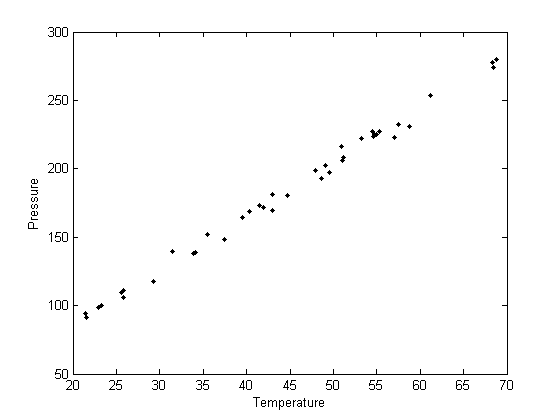
plot(T,P,'k. ')
xlabel('Temperature')
ylabel('Pressure')

Fit a line to the data for P(T) = a + bT

It appears the data is roughly linear, and we know from the ideal gas law that PV = nRT, or P = nR/V*T, which says P should be linearly correlated with V. Note that the temperature data is in degC, not in K, so it is not expected that P=0 at T = 0. let X = T, and Y = P for the regress syntax. The regress command expects a column of ones for the constant term so that the statistical tests it performs are valid. We get that column by raising the independent variable to the zero power.

X = [T.^0 T]; % [1 T1]
Y = P;
alpha = 0.05; % specifies the 95% confidence interval

[b bint] = regress(Y,X,alpha)

b =

    7.7490
    3.9301


bint =

    2.9839   12.5141
    3.8275    4.0328

Note that the intercept is not zero, although, the confidence interval is fairly large, it does not include zero at the 95% confidence level.

Calculate R^2 for the line

The R^2 value accounts roughly for the fraction of variation in the data that can be described by the model. Hence, a value close to one means nearly all the variations are described by the model, except for random variations.

ybar = mean(Y);
SStot = sum((Y - ybar).^2);
SSerr = sum((Y - X*b).^2);
R2 = 1 - SSerr/SStot;
sprintf('R^2 = %1.3f',R2)

ans =

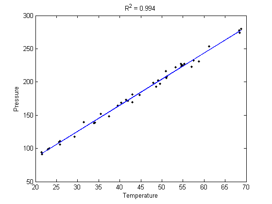
R^2 = 0.994

Plot the data and the fit

plot(T,P,'k. ',T,X*b,'b -')
xlabel('Temperature')
ylabel('Pressure')
title(sprintf('R^2 = %1.3f',R2))

Evaluating the model

The fit looks good, and R^2 is near one, but is it a good model? There are a few ways to examine this. We want to make sure that there are no systematic trends in the errors between the fit and the data, and we want to make sure there are not hidden correlations with other variables.

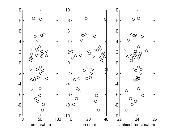
Plot the residuals

the residuals are the error between the fit and the data. The residuals should not show any patterns when plotted against any variables, and they do not in this case.

residuals = P - X*b;
figure
hold all
subplot(1,3,1)
plot(T,residuals,'ko')
xlabel('Temperature')

subplot(1,3,2)
plot(run_order,residuals,'ko ')
xlabel('run order')

subplot(1,3,3)
plot(ambientT,residuals,'ko')
xlabel('ambient temperature')

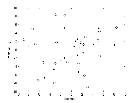
check for correlations between residuals

We assume all the errors are uncorrelated with each other. We use a lag plot, where we plot residual(i) vs residual(i-1), i.e. we look for correlations between adjacent residuals. This plot should look random, with no correlations if the model is good.

figure
plot(residuals(2:end),residuals(1:end-1),'ko')
xlabel('residual(i)')
ylabel('residual(i-1)')

Alternative models

Lets consider a quadratic model instead.

X = [T.^0 T.^1 T.^2];
Y = P;
alpha = 0.05; % 95% confidence interval

[b bint] = regress(Y,X,alpha)

b =

    9.0035
    3.8667
    0.0007


bint =

   -4.7995   22.8066
    3.2046    4.5288
   -0.0068    0.0082

You can see that the 95% confidence interval on the constant and includes zero, so adding a parameter does not increase the goodness of fit. This is an example of overfitting the data, but it also makes you question whether the constant is meaningful in the linear model. The regress function expects a constant in the model, and the documentation says leaving it out

Alternative models

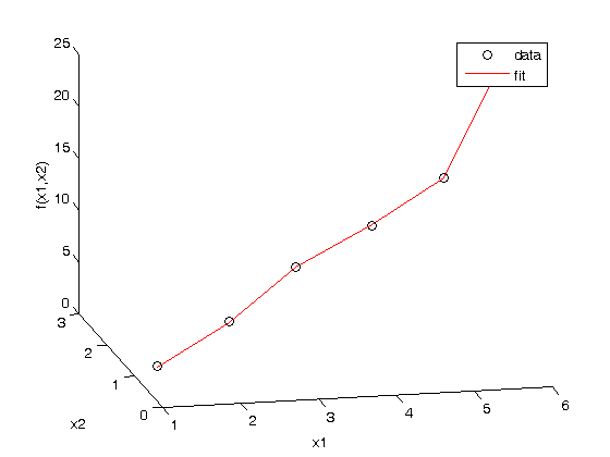
Lets consider a model with intercept = 0, P = alpha*T

X = [T];
Y = P;
alpha = 0.05; % 95% confidence interval

[b bint] = regress(Y,X,alpha)
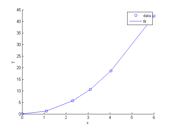
plot(T,P,'k. ',T,X*b,'b- ')
xlabel('Temperature')
ylabel('Pressure')
legend 'data' 'fit'

ybar = mean(Y);
SStot = sum((Y - ybar).^2);
SSerr = sum((Y - X*b).^2);
R2 = 1 - SSerr/SStot;
title(sprintf('R^2 = %1.3f',R2))

b =

    4.0899


bint =

    4.0568    4.1231

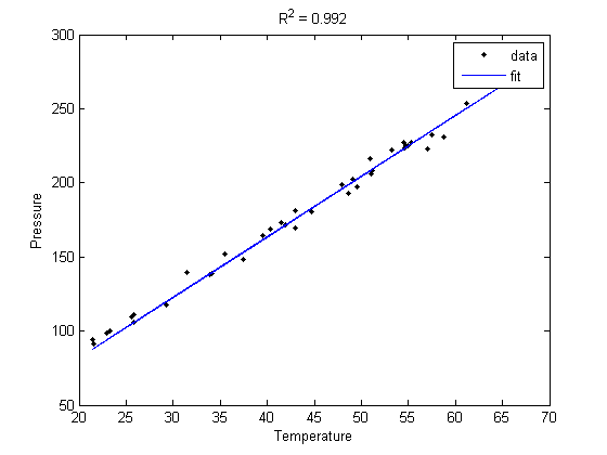
The fit is visually still good. and the R^2 value is only slightly worse.

plot residuals

You can see a slight trend of decreasing value of the residuals as the Temperature increases. This may indicate a deficiency in the model with no intercept. For the ideal gas law in degC: 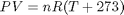or , so the intercept is expected to be non-zero in this case. That is an example of the deficiency.

residuals = P - X*b;
figure
plot(T,residuals,'ko')
xlabel('Temperature')
ylabel('residuals')

'done'
% categories: data analysis

ans =

done

Published with MATLAB® 7.12

Contents

Fitting a numerical ODE solution to data

function main

clc; clear all; close all

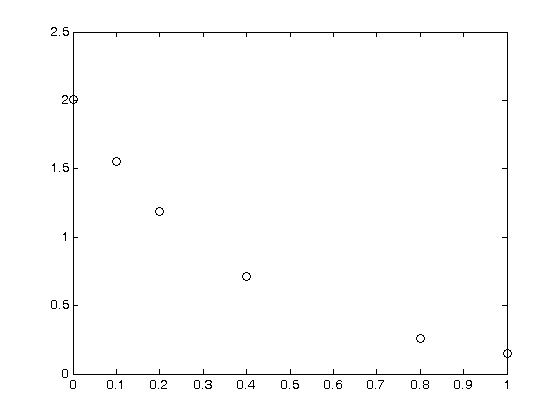
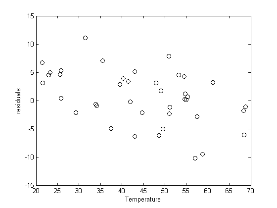
Suppose we know the concentration of A follows this differential equation: , and we have the following data:

Lets make these column vectors

tspan = [0 0.1 0.2 0.4 0.8 1]';
Ca_data = [2.0081  1.5512  1.1903  0.7160  0.2562  0.1495]';
plot(tspan,Ca_data,'ko ')

In this case, one could solve the simple ODE, and transform the data to get a simple linear fit. Instead, we are going to develop a method to directly fit the ODE solution to the data.

parguess = [1.3]; % nonlinear fits need initial guesses
[pars, resid, J] = nlinfit(tspan,Ca_data,@myfunc,parguess)

pars =

    2.5889


resid =

         0
    0.0011
   -0.0062
    0.0031
    0.0031
   -0.0013


J =

         0
   -0.1550
   -0.2393
   -0.2852
   -0.2025
   -0.1508

the residuals are pretty low. J is a Jacobian, and we don't need to worry about it. It is used to estimate confidence intervals.

parameter confidence intervals

alpha = 0.05; % this is for 95% confidence intervals
pars_ci = nlparci(pars,resid,'jacobian',J,'alpha',alpha)

sprintf('The true value of k is between %1.2f and %1.2f at the 95%% confidence level',pars_ci)

pars_ci =

    2.5701    2.6077


ans =

The true value of k is between 2.57 and 2.61 at the 95% confidence level

now we can examine the fit

tfit = linspace(0,1);
fit = myfunc(pars,tfit);
hold all
plot(tfit,fit)

You can see the fit looks ok. To summarize, here is a way to directly fit an ODE solution to data using the nonlinear fitting algorithms of Matlab. The advantage of this over a transformation, e.g. by computing the derivative or by plotting log(Ca/Cao) vs. something is that this approach avoids the nonlinear transformation of errors in the data. That comes at the expense of having to solve a nonlinear problem which requires an initial guess. Sometimes, that can be hard.

function to fit

This is the function we want to fit to the data. When we have the right pars, the output of this function should be a close fit to the data above. We use a nested function in a nested function to avoid needing lots of function handles to pass parameters around.

    function output = myfunc(pars,tspan)
        % we just rename the variable here for use in the ODE
        k = pars;
            function dCadt = ode(t,Ca)
                % this is the ODE we are fitting to
                dCadt = -k*Ca;
            end
        % we use the actual tspan data to get the solution to the ode at
        % the right points.
        Cao = Ca_data(1);
        [t,Ca] = ode45(@ode,tspan,Cao);
        output = Ca;
    end % myfunc

end % main

% categories: data analysis

Published with MATLAB® 7.12

Linear least squares fitting with linear algebra

John Kitchin

clear all; clc; close all
% Given this data, we want to fit a line to the data to extract the slope.
u = cmu.units;
x = [0 0.5 1 1.5 2 3 4 6 10]*u.s;  % time
y = [0 -0.157 -0.315 -0.472 -0.629 -0.942 -1.255 -1.884 -3.147]*u.dimensionless; % dimensionless

figure
plot(x,y,'bo ')

The nature of this method is that we can write a series of equations:

x1^0*b0 + x1*b1 = y1
x2^0*b0 + x2*b1 = y2
x3^0*b0 + x3*b1 = y3
etc...

Which we can write in matrix form: X b = y.

where X is a matrix of column vectors like this:

X = [(x.^0)' x']

matrix with mixed row or column units

ans =

    1.0000         0
    1.0000    0.5000
    1.0000    1.0000
    1.0000    1.5000
    1.0000    2.0000
    1.0000    3.0000
    1.0000    4.0000
    1.0000    6.0000
    1.0000   10.0000

We cannot solve for the unknowns b, because the X matrix is not square. There are many more rows in X than in B. to make X square, we left multiply each side by transpose(X) to get

X^T X b = X^T y

then we can use the Matlab syntax with the backslash operator that solves linear equations

b = (X'*X)\(X'*y')
b2 = b(2)

|0.00|
-0.31|
-0.314522

or even more directly, since the backslash operator solves in the least squares sense if there are more rows than columns. Note these only work for linear equations!

b = X\y'
b2 = b(2)

matrix with mixed row or column units

ans =

    0.0006
   -0.3145

-0.314522/s

the intercept is b(1), and the slope is b(2). We can make a simple function of the fit, and plot it on the data.

fit = @(z) b(1) + b(2)*z;
hold all
h = plot(x, X*b, 'r- ');

this method can be readily extended to fitting any polynomial model, or other linear model that is fit in a least squares sense. This method does not provide confidence intervals, as the related method discussed in Post 943 using the regress command, but it is probably how that method does the fitting.

'done'

% categories: data analysis
% post_id = 1141; %delete this line to force new post;

ans =

done

Published with MATLAB® 7.12