Nonlinear curve fitting with parameter confidence intervals

| categories: data analysis | View Comments

L11_2b

Contents

Nonlinear curve fitting with parameter confidence intervals

John Kitchin

clear all; close all; clc

raw data to fit

x = [0.5 0.387 0.24 0.136 0.04 0.011];
y = [1.255 1.25 1.189 1.124 0.783 0.402];
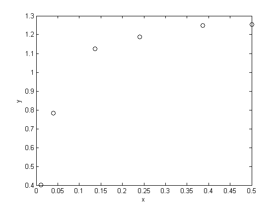
plot the data

you should usually plot your data to get a feel for how it looks.

plot(x,y,'ko')
xlabel('x')
ylabel('y')

nonlinear fitting

fit this nonlinear model y = Ax/(B+x) to the data. I use a function handle here, but I think it is cleaner and easier to read with a subfunction. here pars(1) = A, and pars(2) = B

f = @(pars,x) pars(1)*x./(pars(2)+x);

parguess = [ 1.3 0.03]; % nonlinear fits need initial guesses
[pars, resid, J] = nlinfit(x,y,f,parguess)
pars =

    1.3275    0.0265


resid =

   -0.0058    0.0074   -0.0067    0.0127   -0.0160    0.0122


J =

    0.9497   -2.3949
    0.9360   -3.0053
    0.9007   -4.4873
    0.8371   -6.8404
    0.6019  -12.0216
    0.2936  -10.4056

get the confidence interval for each parameter

the nlparci command estimates confidence intervals. The first row of the output is parameter 1, second row parameter 2, ...

alpha = 0.05; % this is for 95% confidence intervals
pars_ci = nlparci(pars,resid,'jacobian',J,'alpha',alpha)
sprintf('A is in the range of [%1.2f %1.2f] at the 95%% confidence level',pars_ci(1,:))
sprintf('B is in the range of [%1.2f %1.2f] at the 95%% confidence level',pars_ci(2,:))
pars_ci =

    1.3005    1.3545
    0.0236    0.0293


ans =

A is in the range of [1.30 1.35] at the 95% confidence level


ans =

B is in the range of [0.02 0.03] at the 95% confidence level

hold all
xfit = linspace(0.5, 0.011);
plot(xfit,f(pars,xfit),'DisplayName','fitted model')
legend show
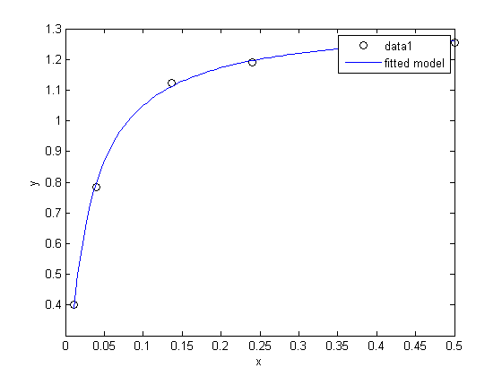
summary

The fit looks reasonable, and the confidence intervals are "tight" and do not include zero, suggesting the parameters are significant.

% categories: data analysis
Read and Post Comments

Linear regression with confidence intervals.

| categories: data analysis | View Comments

Linear regression with confidence intervals.

Linear regression with confidence intervals.

Fit a fourth order polynomial to this data and determine the confidence interval for each parameter. Data from example 5-1 in Fogler, Elements of Chemical Reaction Engineering

Contents

data to fit

note the transpose so these are column vectors

t = [0 50 100 150 200 250 300]';
Ca = [50 38 30.6 25.6 22.2 19.5 17.4]'*1e-3;

We want the equation $Ca(t) = b0 + b1*t + b2*t^2 + b3*t^3 + b4*t^4$ 
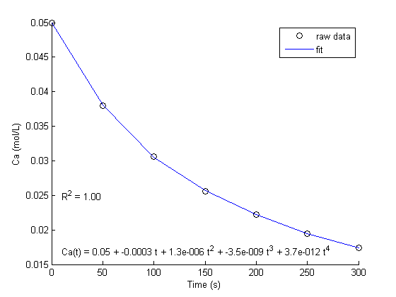
fit to the data in the least squares sense. We can write this in a linear algebra form as: T*b = Ca where T is a matrix of columns [1 t t^2 t^3 t^4], and b is a column vector of [b0 b1 b2 b3 b4]'. We want to solve for the b vector.

T = [ones(size(t)) t t.^2 t.^3 t.^4];

% we use the :command:`regress` to solve for b
alpha = 0.05 % confidence interval is 100*(1 - alpha)
[b,bint] = regress(Ca,X, alpha)
% b is the solution to our equation
% bint is the 95% confidence interval for each parameter

% the numbers are a little small to see with the default format
alpha =

    0.0500


b =

    0.0500
   -0.0003
    0.0000
   -0.0000
    0.0000


bint =

    0.0497    0.0503
   -0.0003   -0.0003
    0.0000    0.0000
   -0.0000   -0.0000
    0.0000    0.0000

change the format to see the numbers

format long
b
bint
% this lets you see 15 decimal places, but alot of them are zeros.
b =

   0.049990259740260
  -0.000297846320346
   0.000001343484848
  -0.000000003484848
   0.000000000003697


bint =

   0.049680246760215   0.050300272720305
  -0.000315461979157  -0.000280230661536
   0.000001071494761   0.000001615474936
  -0.000000004903197  -0.000000002066500
   0.000000000001350   0.000000000006044

engineering format

format shorte
b
bint
b =

  4.9990e-002
 -2.9785e-004
  1.3435e-006
 -3.4848e-009
  3.6970e-012


bint =

  4.9680e-002  5.0300e-002
 -3.1546e-004 -2.8023e-004
  1.0715e-006  1.6155e-006
 -4.9032e-009 -2.0665e-009
  1.3501e-012  6.0439e-012

compute R^2

http://en.wikipedia.org/wiki/Coefficient_of_determination

format % set format back to normal
SS_tot = sum((Ca - mean(Ca)).^2);
SS_err = sum((X*b - Ca).^2);

Rsq = 1 - SS_err/SS_tot
Rsq =

    1.0000

Plot the data and the fit

hold on
plot(t,Ca,'ko ','DisplayName','raw data')
plot(t,X*b,'b ','DisplayName','fit')
legend show
xlabel('Time (s)')
ylabel('Ca (mol/L)')

text(10,0.025,sprintf('R^2 = %1.2f',Rsq))
text(10,0.017,sprintf('Ca(t) = %1.2g + %1.2g t + %1.2g t^2 + %1.2g t^3 + %1.2g t^4',b))

Summary

a fourth order polynomial fits the data well, with a good R^2 value. All of the parameters appear to be significant, i.e. zero is not included in any of the parameter confidence intervals. This does not mean this is the best model for the data, just that the model fits well.

'done'

% categories: Data analysis
ans =

done

Read and Post Comments

Introduction to statistical data analysis

| categories: data analysis | View Comments

statistics

Contents

Introduction to statistical data analysis

clear all
clc

Problem statement.

Given several measurements of a single quantity, determine the average value of the measurements, the standard deviation of the measurements and the 95% confidence interval for the average.

the data

y = [8.1 8.0 8.1];

the average and standard deviation

ybar = mean(y)
s = std(y)
ybar =

    8.0667


s =

    0.0577

the confidence interval

This is a recipe for computing the confidence interval. The strategy is:
  1. compute the average
  2. Compute the standard deviation of your data
  3. Define the confidence interval, e.g. 95% = 0.95
  4. compute the student-t multiplier. This is a function of the confidence interval you specify, and the number of data points you have minus 1. You subtract 1 because one degree of freedom is lost from calculating the average.

The confidence interval is defined as ybar +- T_multiplier*std/sqrt(n).

the tinv command provides the T_multiplier

ci = 0.95;
alpha = 1 - ci;

n = length(y); %number of elements in the data vector
T_multiplier = tinv(1-alpha/2, n-1)
% the multiplier is large here because there is so little data. That means
% we do not have a lot of confidence on the true average or standard
% deviation
ci95 = T_multiplier*s/sqrt(n)

% confidence interval
sprintf('The confidence interval is %1.1f +- %1.1f',ybar,ci95)
[ybar - ci95, ybar + ci95]

% we can say with 95% confidence that the true mean lies between these two
% values.

% categories: Data analysis
T_multiplier =

    4.3027


ci95 =

    0.1434


ans =

The confidence interval is 8.1 +- 0.1


ans =

    7.9232    8.2101

Read and Post Comments

Fit a line to numerical data

| categories: data analysis | View Comments

Fit a line to numerical data

Fit a line to numerical data

John Kitchin

Contents

Problem statement

fit a line to this data

x = [0 0.5 1 1.5 2.0 3.0 4.0 6.0 10];
y = [0 -0.157 -0.315 -0.472 -0.629 -0.942 -1.255 -1.884 -3.147];

polyfit(x,y,n) where n is the polynomial order, n=1 for a line

note that the output of this command is a "polynomial in Matlab. See polynomials for more details.

p = polyfit(x,y,1)

slope=p(1)
intercept=p(2)
p =

   -0.3145    0.0006


slope =

   -0.3145


intercept =

  6.2457e-004

we can calculate the fitted values with polyval

fittedy = polyval(p,x);

or by hand

fittedy2 = slope*x + intercept;

plot each method for comparison

figure(1)
hold on
plot(x,y,'ro','DisplayName','raw data')
plot(x,fittedy,'k-','DisplayName','fit from polyval')
plot(x,fittedy2,'y-- ','DisplayName','fit from equation by hand')
xlabel('x')
ylabel('y')
legend show
% These should be indistinguishable. We use combinations of symbols with no
% lines, solid lines, and dashed lines to see that all curves are the same.

% categories: Data analysis
% tags: math
% post_id = 650; %delete this line to force new post;
Read and Post Comments

« Previous Page