Linear regression with confidence intervals.

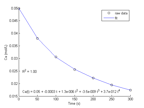
Fit a fourth order polynomial to this data and determine the confidence interval for each parameter. Data from example 5-1 in Fogler, Elements of Chemical Reaction Engineering

Contents

data to fit

note the transpose so these are column vectors

t = [0 50 100 150 200 250 300]';
Ca = [50 38 30.6 25.6 22.2 19.5 17.4]'*1e-3;

We want the equation fit to the data in the least squares sense. We can write this in a linear algebra form as: T*b = Ca where T is a matrix of columns [1 t t^2 t^3 t^4], and b is a column vector of [b0 b1 b2 b3 b4]'. We want to solve for the b vector.

T = [ones(size(t)) t t.^2 t.^3 t.^4];

% we use the :command:`regress` to solve for b
alpha = 0.05 % confidence interval is 100*(1 - alpha)
[b,bint] = regress(Ca,X, alpha)
% b is the solution to our equation
% bint is the 95% confidence interval for each parameter

% the numbers are a little small to see with the default format

alpha =

    0.0500


b =

    0.0500
   -0.0003
    0.0000
   -0.0000
    0.0000


bint =

    0.0497    0.0503
   -0.0003   -0.0003
    0.0000    0.0000
   -0.0000   -0.0000
    0.0000    0.0000

change the format to see the numbers

format long
b
bint
% this lets you see 15 decimal places, but alot of them are zeros.

b =

   0.049990259740260
  -0.000297846320346
   0.000001343484848
  -0.000000003484848
   0.000000000003697


bint =

   0.049680246760215   0.050300272720305
  -0.000315461979157  -0.000280230661536
   0.000001071494761   0.000001615474936
  -0.000000004903197  -0.000000002066500
   0.000000000001350   0.000000000006044

engineering format

format shorte
b
bint

b =

  4.9990e-002
 -2.9785e-004
  1.3435e-006
 -3.4848e-009
  3.6970e-012


bint =

  4.9680e-002  5.0300e-002
 -3.1546e-004 -2.8023e-004
  1.0715e-006  1.6155e-006
 -4.9032e-009 -2.0665e-009
  1.3501e-012  6.0439e-012

compute R^2

http://en.wikipedia.org/wiki/Coefficient_of_determination

format % set format back to normal
SS_tot = sum((Ca - mean(Ca)).^2);
SS_err = sum((X*b - Ca).^2);

Rsq = 1 - SS_err/SS_tot

Rsq =

    1.0000

Plot the data and the fit

hold on
plot(t,Ca,'ko ','DisplayName','raw data')
plot(t,X*b,'b ','DisplayName','fit')
legend show
xlabel('Time (s)')
ylabel('Ca (mol/L)')

text(10,0.025,sprintf('R^2 = %1.2f',Rsq))
text(10,0.017,sprintf('Ca(t) = %1.2g + %1.2g t + %1.2g t^2 + %1.2g t^3 + %1.2g t^4',b))

Summary

a fourth order polynomial fits the data well, with a good R^2 value. All of the parameters appear to be significant, i.e. zero is not included in any of the parameter confidence intervals. This does not mean this is the best model for the data, just that the model fits well.

'done'

% categories: Data analysis

ans =

done

Published with MATLAB® 7.12