Interpolation of data

| categories: basic matlab | View Comments

interpolation

Contents

Interpolation of data

when we have data at two points but we need data in between them we use interpolation. Suppose we have the points (4,3) and (6,2) and we want to know the value of y at x=4.65, assuming y varies linearly between these points. we use the interp1 command to achieve this.

x = [4 6]
y = [3 2]

interp1(x,y,4.65)
x =

     4     6


y =

     3     2


ans =

    2.6750

multiple interpolation values

you can interpolate several values

interp1(x,y,[4.65 5.01 4.2 9])
% note that you cannot interpolate outside the region where data is
% defined. That is why the value at x=9 is NaN.
ans =

    2.6750    2.4950    2.9000       NaN

more sophisticated interpolation.

the default interpolation method is simple linear interpolation between points. Other methods exist too, such as fitting a spline to the data and using the spline representation to interpolate from.

x = [1 2 3 4];
y = [1 4 9 16]; % y = x^2
xi = [ 1.5 2.5 3.5]; % we want to interpolate on these values
y1 = interp1(x,y,xi);
y2 = interp1(x,y,xi,'spline')
y2 =

    2.2500    6.2500   12.2500

Compare these methods by plotting each set of interpolated values

the data we interpolated was constructed from y = x^2

figure
hold on
ezplot('x^2',[1 4])
plot(xi,y1,'rs',xi,y2,'bd')
legend('data','linear interpolation','spline interpolation')
hold off
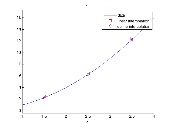
summary: in this case the spline interpolation is a little more accurate than the linear interpolation. That is because the underlying data was polynomial in nature, and a spline is like a polynomial. That may not always be the case, and you need some engineering judgement to know which method is best.

% categories: Basic Matlab
% tags: math
Read and Post Comments

Integrating functions in Matlab

| categories: basic matlab | View Comments

integrate_functions

Contents

Integrating functions in Matlab

it is a good idea to add these lines to the top of your m-files. They keep things looking neat!

close all  % close all figure windows that are open
clear all  % clear all the variables currently stored in memory
clc        % clear the commands in the command window

Problem statement

find the integral of a function f(x) from a to b i.e.

$$\int_a^b f(x) dx$$

In matlab we use numerical quadrature to achieve this with the `quad` command. f = @(x) some_function_of_x quad(f,a,b)

as a specific example, lets integrate

$$y=x^2$$

from x=0 to x=1. You should be able to work out that the answer is 1/3.

f = @(x) x.^2;  %note we must use .^ to ensure element-wise squaring
a = 0;
b = 1;

integrand = quad(f,a,b)
integrand =

    0.3333

double integrals

we use the `dblquad` command

Integrate $f(x,y)=y sin(x)+x cos(y)$ over

$\pi <= x <= 2\pi$

$0 <= y <= \pi$

i.e.

$\int_{x=\pi}^{2\pi}\int_{y=0}^{\pi}y sin(x)+x cos(y)dydx$

f = @(x,y) y*sin(x)+x*cos(y);
x1=pi; x2=2*pi;
y1=0; y2=pi;
integrand = dblquad(f, x1,x2,y1,y2)
integrand =

   -9.8696

triple integrals

we use the `triplequad` command Integrate $f(x,y,z)=y sin(x)+z cos(x)$ over the region

$0 <= x <= \pi$

$0 <= y <= 1$

$-1 <= z <= 1$

f = @(x,y,z) y*sin(x)+z*cos(x);
x1=0; x2=pi;
y1=0; y2=1;
z1=-1; z2=1;
integrand = triplequad(f, x1,x2,y2,y2,z1,z2)

% categories: Basic matlab
% tags: math
integrand =

     0

Read and Post Comments

Illustrating matrix transpose rules in matrix multiplication

| categories: linear algebra | View Comments

Illustrating matrix transpose rules in matrix multiplication

Illustrating matrix transpose rules in matrix multiplication

John Kitchin

Contents

Rules for transposition

Here are the four rules for matrix multiplication and transposition

1. $(\mathbf{A}^T)^T = \mathbf{A}$

2. $(\mathbf{A}+\mathbf{B})^T = \mathbf{A}^T+\mathbf{B}^T$

3. $(\mathit{c}\mathbf{A})^T = \mathit{c}\mathbf{A}^T$

4. $(\mathbf{AB})^T = \mathbf{B}^T\mathbf{A}^T$

reference: Chapter 7.2 in Advanced Engineering Mathematics, 9th edition. by E. Kreyszig.

The transpose in Matlab

there are two ways to get the transpose of a matrix: with a notation, and with a function

A = [[5 -8 1];
    [4 0 0]]
A =

     5    -8     1
     4     0     0

function

transpose(A)
ans =

     5     4
    -8     0
     1     0

notation

A.'

% note, these functions only provide the non-conjugate transpose. If your
% matrices are complex, then you want the ctranspose function, or the
% notation A' (no dot before the apostrophe). For real matrices there is no
% difference between them.

% below we illustrate each rule using the different ways to get the
% transpose.
ans =

     5     4
    -8     0
     1     0

Rule 1

m1 = (A.').'
A

all(all(m1 == A)) % if this equals 1, then the two matrices are equal
m1 =

     5    -8     1
     4     0     0


A =

     5    -8     1
     4     0     0


ans =

     1

Rule 2

B = [[3 4 5];
    [1 2 3]];
m1 = transpose(A+B)
m2 = transpose(A) + transpose(B)

all(all(m1 == m2)) % if this equals 1, then the two matrices are equal
m1 =

     8     5
    -4     2
     6     3


m2 =

     8     5
    -4     2
     6     3


ans =

     1

Rule 3

c = 2.1;
m1 = transpose(c*A)
m2 = c*transpose(A)

all(all(m1 == m2)) % if this equals 1, then the two matrices are equal
m1 =

   10.5000    8.4000
  -16.8000         0
    2.1000         0


m2 =

   10.5000    8.4000
  -16.8000         0
    2.1000         0


ans =

     1

Rule 4

B = [[0 2];
    [1 2];
    [6 7]]

m1 = (A*B).'
m2 = B.'*A.'

all(all(m1 == m2)) % if this equals 1, then the two matrices are equal
B =

     0     2
     1     2
     6     7


m1 =

    -2     0
     1     8


m2 =

    -2     0
     1     8


ans =

     1

m3 = A.'*B.'
% you can see m3 has a different shape than m1, so there is no way they can
% be equal.
m3 =

     8    13    58
     0    -8   -48
     0     1     6

% categories: Linear algebra
% tags: math
% post_id = 552; %delete this line to force new post;
Read and Post Comments

« Previous Page