transient heat conduction - partial differential equations

adapated from http://msemac.redwoods.edu/~darnold/math55/DEproj/sp02/AbeRichards/slideshowdefinal.pdf

Contents

In Post 860 we solved a steady state BVP modeling heat conduction. Today we examine the transient behavior of a rod at constant T put between two heat reservoirs at different temperatures, again T1 = 100, and T2 = 200. The rod will start at 150. Over time, we should expect a solution that approaches the steady state solution: a linear temperature profile from one side of the rod to the other.

at , in this example we have as an initial condition. with boundary conditions and .

Matlab provides the pdepe command which can solve some PDEs. The syntax for the command is

 sol = pdepe(m,@pdex,@pdexic,@pdexbc,x,t)

where m is an integer that specifies the problem symmetry. The three function handles define the equations, initial conditions and boundary conditions. x and t are the grids to solve the PDE on.

function pdexfunc

close all; clc; clear all;

setup the problem

m=0; % specifies 1-D symmetry
x = linspace(0,1); % equally-spaced points along the length of the rod
t = linspace(0,5); % this creates time points

sol = pdepe(m,@pdex,@pdexic,@pdexbc,x,t);

plot the solution as a 3D surface

x is the position along the rod, t is the time sol is the temperature at (x,t)

surf(x,t,sol)
xlabel('Position')
ylabel('time')
zlabel('Temperature')

in the surface plot above you can see the approach from the initial conditions to the steady state solution.

we can also plot the solutions in 2D, at different times. Our time vector has about 100 elements, so in this loop we plot every 5th time. We set a DisplayName in each plot so we can use them in the legend later.

figure
hold all % the use of all makes the colors cycle with each plot
for i=1:5:numel(t)
    plot(x,sol(i,:),'DisplayName',sprintf('t = %1.2f',t(i)))
end
xlabel('length')
ylabel('Temperature')

% we use -DynamicLegend to pick up the display names we set above.
legend('-DynamicLegend','location','bestoutside');
% this is not an easy way to see the solution.

animating the solution

we can create an animated gif to show how the solution evolves over time.

filename = 'animated-solution.gif'; % file to store image in
for i=1:numel(t)
    plot(x,sol(i,:));
    xlabel('Position')
    ylabel('Temperature')
    text(0.1,190,sprintf('t = %1.2f',t(i))); % add text annotation of time step
    frame = getframe(1);
    im = frame2im(frame); %convert frame to an image
    [imind,cm] = rgb2ind(im,256);

    % now we write out the image to the animated gif.
    if i == 1;
        imwrite(imind,cm,filename,'gif', 'Loopcount',inf);
    else
        imwrite(imind,cm,filename,'gif','WriteMode','append');
    end
end
close all; % makes sure the plot from the loop above doesn't get published

here is the animation!

It is slightly more clear that the temperature profile evolves from a flat curve, to a linear temperature ramp between the two end points.

'done'

ans =

done

function [c,f,s] = pdex(x,t,u,DuDx)

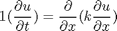
For pdepe to understand the equations, they need to be in the form of

where c is a diagonal matrix, f is called a flux term, and s is the source term. Our equations are:

from which you can see that , , and

c = 1;
f = 0.02*DuDx;
s = 0;

function u0 = pdexic(x)
% this defines u(t=0) for all of x. The problem specifies a constant T for
% all of x.
u0 = 150;

function [p1,q1,pr,qr] = pdexbc(x1,u1,xr,ur,t)
% this defines the boundary conditions. The general form of the boundary
% conditions are $p(x,t,u) + q(x,t)f(x,t,u,\frac{\partial u}{\partial x})$
% We have to define the boundary conditions on the left, and right.
p1 = u1-100; % at left
q1 = 0; % at left
pr= ur-200;  % at right
qr = 0; % at right


% categories: PDEs
% tags: heat transfer

Published with MATLAB® 7.10

Boundary value problem in heat conduction

For steady state heat conduction the temperature distribution in one-dimension is governed by the Laplace equation:

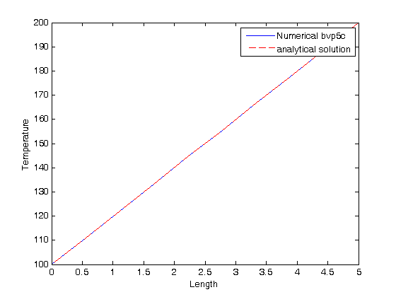
with boundary conditions that at and . To solve this in Matlab, we need to convert the second order differential equation into a system of first order ODEs, and use the bvp5c command to get a numerical solution.

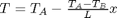the analytical solution is not difficult here: . but the bvp5c syntax takes a lot to get used to.

For this problem, lets consider a slab that is defined by x=0 to x=L, with T(x=0) = 100, and T(x=L) = 200. We want to find the function T(x) inside the slab.

To get the system of ODEs, let , and . That leads to and the following set of equations:

with boundary conditions and . By inspection you can see that whatever value has, it will remain constant since the derivative of is equal to zero.

function main

we start by defining an initial grid to get the solution on

x = linspace(0,5,10);

Next, we use the bvpinit command to provide an initial guess using the guess function defined below

solinit = bvpinit(x,@guess);

we also need to define the ode function (see odefun below).

and a boundary condition function (see bcfun below).

now we can get the solution.

sol = bvp5c(@odefun,@bcfun,solinit)

sol = 

    solver: 'bvp5c'
         x: [0 0.5556 1.1111 1.6667 2.2222 2.7778 3.3333 3.8889 4.4444 5]
         y: [2x10 double]
     idata: [1x1 struct]
     stats: [1x1 struct]

sol is a Matlab struct with fields. the x field contains the x-values of the solution as a row vector, the y field contains the solutions to the odes. Recall that T1 is the only solution we care about, as it is the original T(x) we were interested in.

x = sol.x;
T1 = sol.y(1,:);
T2 = sol.y(2,:);
plot(x,T1); figure(gcf)
xlabel('Length')
ylabel('Temperature')

% for demonstration we add the analytical solution to the plot
hold on
Ta = 100; Tb = 200; L = 5;
plot(x,Ta - (Ta-Tb)/L*x,'r--')
legend 'Numerical bvp5c' 'analytical solution'

As we would expect, the solutions agree, and show that the temperature changes linearly from the temperature at x=0 to the temperature at x=L.

the stats field gives you some information about the solver, number of function evaluations and maximum errors

sol.stats

ans = 

    nmeshpoints: 10
         maxerr: 9.8021e-016
      nODEevals: 106
       nBCevals: 9

function Tinit = guess(x)
% this is an initial guess of the solution. We need to provide a guess of
% what the function values of T1(x) and T2(x) are for a value of x. In some
% cases, this initial guess may affect the ability of the solver to get a
% solution. In this example, we guess that T1 is a constant and average
% value between 100 and 200. In this example, it also does not matter what
% T2 is, because it never changes.
T1 = 150;
T2 = 1;
Tinit = [T1; T2]; % we return a column vector

function dTdx = odefun(x,T)
% here we define our differential equations
T1 = T(1);
T2 = T(2);

dT1dx = T2;
dT2dx = 0;

dTdx = [dT1dx; dT2dx];

function res = bcfun(T_0,T_L)
% this function defines the boundary conditions for each ode. In this
% example, T_O = [T1(0)  T2(0)], and T_L = [T1(L) T2(L)]. The function
% computes a residual, which is the difference of what the current solution
% at the boundary conditions are vs. what they are supposed to be.  We want
% T1(0) = 100; and T1(L)=200. There are no requirements on the boundary
% values for T2 in this example.
res = [100 - T_0(1);
       200 - T_L(1)];

% categories: ODEs
% tags: math, heat transfer

Published with MATLAB® 7.10