Boundary value problem in heat conduction

For steady state heat conduction the temperature distribution in one-dimension is governed by the Laplace equation:

with boundary conditions that at and . To solve this in Matlab, we need to convert the second order differential equation into a system of first order ODEs, and use the bvp5c command to get a numerical solution.

the analytical solution is not difficult here: 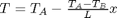. but the bvp5c syntax takes a lot to get used to.

For this problem, lets consider a slab that is defined by x=0 to x=L, with T(x=0) = 100, and T(x=L) = 200. We want to find the function T(x) inside the slab.

To get the system of ODEs, let , and . That leads to and the following set of equations:

with boundary conditions and . By inspection you can see that whatever value has, it will remain constant since the derivative of is equal to zero.

function main

we start by defining an initial grid to get the solution on

x = linspace(0,5,10);

Next, we use the bvpinit command to provide an initial guess using the guess function defined below

solinit = bvpinit(x,@guess);

we also need to define the ode function (see odefun below).

and a boundary condition function (see bcfun below).

now we can get the solution.

sol = bvp5c(@odefun,@bcfun,solinit)

sol = 

    solver: 'bvp5c'
         x: [0 0.5556 1.1111 1.6667 2.2222 2.7778 3.3333 3.8889 4.4444 5]
         y: [2x10 double]
     idata: [1x1 struct]
     stats: [1x1 struct]

sol is a Matlab struct with fields. the x field contains the x-values of the solution as a row vector, the y field contains the solutions to the odes. Recall that T1 is the only solution we care about, as it is the original T(x) we were interested in.

x = sol.x;
T1 = sol.y(1,:);
T2 = sol.y(2,:);
plot(x,T1); figure(gcf)
xlabel('Length')
ylabel('Temperature')

% for demonstration we add the analytical solution to the plot
hold on
Ta = 100; Tb = 200; L = 5;
plot(x,Ta - (Ta-Tb)/L*x,'r--')
legend 'Numerical bvp5c' 'analytical solution'

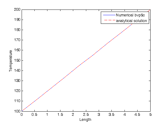
As we would expect, the solutions agree, and show that the temperature changes linearly from the temperature at x=0 to the temperature at x=L.

the stats field gives you some information about the solver, number of function evaluations and maximum errors

sol.stats

ans = 

    nmeshpoints: 10
         maxerr: 9.8021e-016
      nODEevals: 106
       nBCevals: 9

function Tinit = guess(x)
% this is an initial guess of the solution. We need to provide a guess of
% what the function values of T1(x) and T2(x) are for a value of x. In some
% cases, this initial guess may affect the ability of the solver to get a
% solution. In this example, we guess that T1 is a constant and average
% value between 100 and 200. In this example, it also does not matter what
% T2 is, because it never changes.
T1 = 150;
T2 = 1;
Tinit = [T1; T2]; % we return a column vector

function dTdx = odefun(x,T)
% here we define our differential equations
T1 = T(1);
T2 = T(2);

dT1dx = T2;
dT2dx = 0;

dTdx = [dT1dx; dT2dx];

function res = bcfun(T_0,T_L)
% this function defines the boundary conditions for each ode. In this
% example, T_O = [T1(0)  T2(0)], and T_L = [T1(L) T2(L)]. The function
% computes a residual, which is the difference of what the current solution
% at the boundary conditions are vs. what they are supposed to be.  We want
% T1(0) = 100; and T1(L)=200. There are no requirements on the boundary
% values for T2 in this example.
res = [100 - T_0(1);
       200 - T_L(1)];

% categories: ODEs
% tags: math, heat transfer

Published with MATLAB® 7.10