Contents

3D plots of the steam tables

John Kitchin

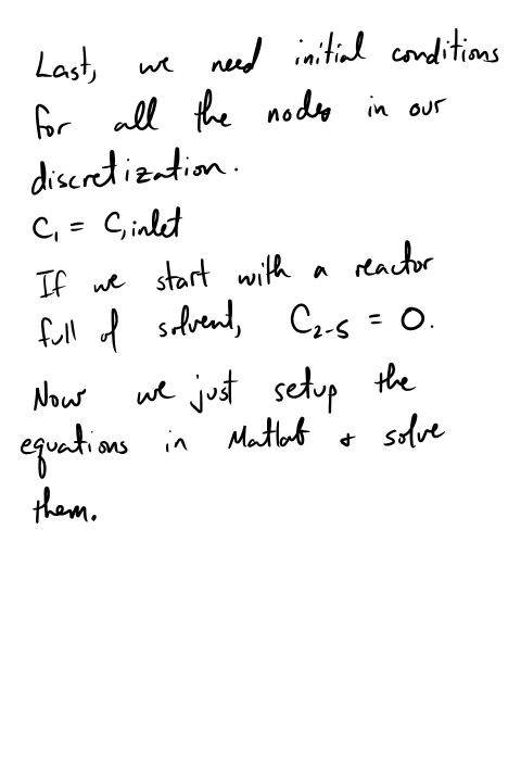
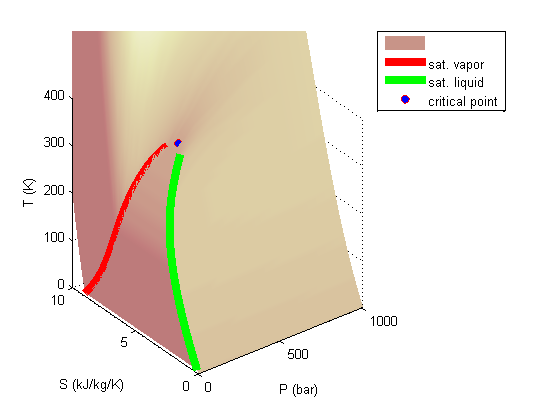
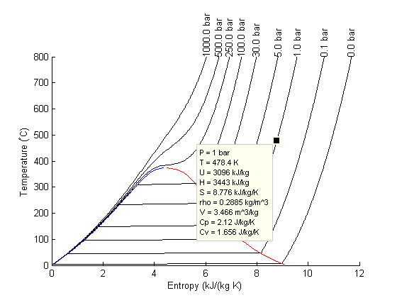
For fun let's make some 3D plots of the steam tables. We will use the XSteam module to map out the pressure, entropy and temperature of steam, and plot the 3D mapping.

clear all; close all; clc

create vectors that we will calculate T for

P = logspace(-2,3); %bar
S = linspace(0,10);

create meshgrid

these are matrices that map out a plane of P,S space

[xdata,ydata] = meshgrid(P,S);
zdata = zeros(size(xdata));

calculate T for each (p,S) pair in the meshgrids

zdata = arrayfun(@(p,s) XSteam('T_ps',p,s),xdata,ydata);

create the 3D plot

we use a lighted surface plot here

surfl(xdata,ydata,zdata)
xlabel('P (bar)')
ylabel('S (kJ/kg/K)')
zlabel('T (K)')
zlim([0 400])

customize the look of the surface plot

this smooths the faces out

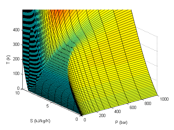
shading interp

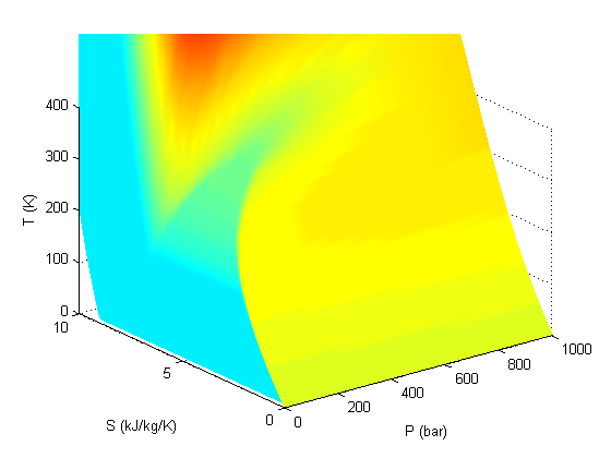
colormap pink

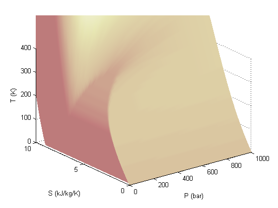
Add the saturated vapor and liquid lines, and the critical point

hold all

Tsat = arrayfun(@(p) XSteam('Tsat_p',p),P);
sV = arrayfun(@(p) XSteam('sV_p',p),P);
sL = arrayfun(@(p) XSteam('sL_p',p),P);
plot3(P,sV,Tsat,'r-','linewidth',5)
plot3(P,sL,Tsat,'g-','linewidth',5)

tc = 373.946; % C
pc = 220.584525; % bar
sc =XSteam('sV_p',pc);
plot3(pc,sc,tc,'ro','markerfacecolor','b') % the critical point
legend '' 'sat. vapor' 'sat. liquid' 'critical point'

Warning: Legend not supported for patches with FaceColor 'interp' 

Summary

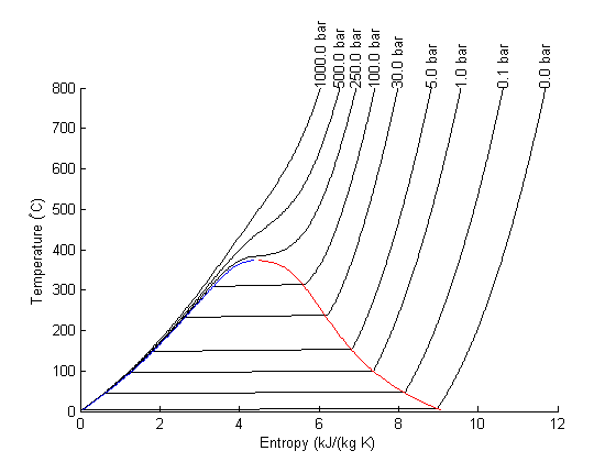
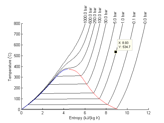
There are lots of options in making 3D plots. They look nice, and from the right perspective can help see how different properties are related. Compare this graph to the one in Post 1484 , where isobars had to be plotted in the 2d graph.

% categories: plotting
% tags: thermodynamics

Published with MATLAB® 7.12

Contents

Interacting with your graph through mouse clicks

John Kitchin

This post continues a series of posts on interacting with Matlab graphs. In Post 1484 we saw an example of customizing a datatip. The limitation of that approach was that you can only click on data points in your graph. Today we examine a way to get similar functionality by defining a function that is run everytime you click on a graph.

You will get a better idea of what this does by watching this short video: http://screencast.com/t/tTm0NlI0eI

function main

close all

Simple contour graph

[X,Y] = meshgrid(-2:.2:2,-2:.2:3);
Z = X.*exp(-X.^2-Y.^2);
[C,h] = contour(X,Y,Z); clabel(C,h);

we can define a function that does something when we click on the graph. We will have the function set the title of the graph to the coordinates of the point we clicked on, and we will print something different depending on which button was pressed. We also want to leave some evidence of where we clicked so it is easy to see. We will put a red plus sign at the point we clicked on.

add an invisible red plus sign to the plot

hold on
cursor_handle = plot(0,0,'r+ ','visible','off')

cursor_handle =

  212.0385

define the callback function

this function will be called for every mouseclick in the axes.

  function mouseclick_callback(gcbo,eventdata)
      % the arguments are not important here, they are simply required for
      % a callback function. we don't even use them in the function,
      % but Matlab will provide them to our function, we we have to
      % include them.
      %
      % first we get the point that was clicked on
      cP = get(gca,'Currentpoint');
      x = cP(1,1);
      y = cP(1,2);
      % Now we find out which mouse button was clicked, and whether a
      % keyboard modifier was used, e.g. shift or ctrl
      switch get(gcf,'SelectionType')
          case 'normal' % Click left mouse button.
              s = sprintf('left: (%1.4g, %1.4g) level = %1.4g',x,y, x.*exp(-x.^2-y.^2));
          case 'alt'    % Control - click left mouse button or click right mouse button.
              s = sprintf('right: (%1.4g, %1.4g level = %1.4g)',x,y, x.*exp(-x.^2-y.^2));
          case 'extend' % Shift - click left mouse button or click both left and right mouse buttons.
              s = sprintf('2-click: (%1.4g, %1.4g level = %1.4g)',x,y, x.*exp(-x.^2-y.^2));
          case 'open'   % Double-click any mouse button.
              s = sprintf('double click: (%1.4g, %1.4g) level = %1.4g',x,y, x.*exp(-x.^2-y.^2));
      end
      % get and set title handle
      thandle = get(gca,'Title');
      set(thandle,'String',s);
      % finally change the position of our red plus, and make it
      % visible.
      set(cursor_handle,'Xdata',x,'Ydata',y,'visible','on')
  end

% now attach the function to the axes
set(gca,'ButtonDownFcn', @mouseclick_callback)

% and we also have to attach the function to the children, in this
% case that is the line in the axes.
set(get(gca,'Children'),'ButtonDownFcn', @mouseclick_callback)

Now, click away and watch the title change!

end

% categories: plotting
% tags: interactive

Published with MATLAB® 7.13

Interacting with the steam Entropy-temperature chart

John Kitchin

Contents

The XSteam module makes it pretty easy to generate figures of the steam tables. Here we generate an entropy-Temperature graph. In :postid:1296` we saw how to generate one of these graphs. In this post, we examine a way to interact with the graph to get more information about each point. In Post 1431 we saw how to use the gname command to add data to datapoints. You can also use the datatip cursor from the toolbar. You could use the standard datatip, but it basically only tells you what you can already see: the entropy and temperature at each point. There was a recent post on one of the Mathwork's blogs on creating a custom datatip, which we will adapt in this post to get all the thermodynamic properties of each data point.

%
function main

close all

Setup the S-T chart

T = linspace(0,800,200); % range of temperatures

fh = figure; % store file handle for later
hold on
% we need to compute S-T for a range of pressures.
pressures = [0.01 0.1 1 5 30 100 250 500 1000]; % bar
for P = pressures
    % XSteam is not vectorized, so here is an easy way to compute a
    % vector of entropies
    S = arrayfun(@(t) XSteam('s_PT',P,t),T);
    plot(S,T,'k-')
    text(S(end),T(end),sprintf('%1.1f bar',P),'rotation',90)
end
% adjust axes positions so the pressure labels don't get cutoff
set(gca,'Position',[0.13 0.11 0.775 0.7])

% plot saturated vapor and liquid entropy lines
svap = arrayfun(@(t) XSteam('sV_T',t),T);
sliq = arrayfun(@(t) XSteam('sL_T',t),T);

plot(svap,T,'r-')
plot(sliq,T,'b-')
xlabel('Entropy (kJ/(kg K)')
ylabel('Temperature (^\circC)')

The regular data tip

Here is what the standard data tip looks like. Not very great! There is so much more information to know about steam. Let's customize the datatip to show all the thermodynamic properties at each point.

Setup the custom output text

we want to display all the thermodynamic properties at each point

    function output_txt = myfunction(obj,event_obj)

        pos = get(event_obj,'Position');
        S = pos(1);
        T = pos(2);
        P = fzero(@(p) XSteam('s_PT',p,T) - S,[0.01 1000]);

        s1 = sprintf('P   = %1.4g bar',P);
        s2 = sprintf('T   = %1.4g K',  T);
        s3 = sprintf('U   = %1.4g kJ/kg', XSteam('u_ps',P,S));
        s4 = sprintf('H   = %1.4g kJ/kg', XSteam('h_ps',P,S));
        s5 = sprintf('S   = %1.4g kJ/kg/K',S);
        s6 = sprintf('rho = %1.4g kg/m^3', XSteam('rho_pT',P,T));
        s7 = sprintf('V   = %1.4g m^3/kg', XSteam('V_pT',P,T));
        s8 = sprintf('Cp  = %1.4g J/kg/K', XSteam('Cp_ps',P,S));
        s9 = sprintf('Cv  = %1.4g J/kg/K', XSteam('Cv_ps',P,S));

        % a cell array of strings makes the output to display in the
        % datatip
        output_txt = {s1; s2; s3; s4; s5; s6; s7; s8; s9};
    end

attach the custom function to the figure

dcm = datacursormode(fh);
set(dcm,'Enable','on');
set(dcm,'updatefcn',@myfunction);
% When published, an extra figure shows up here.

Here is our new datatip.

It looks pretty good! If you move the datatip cursor around, it automatically updates itself.

Summary

Customizing the datatip is a nice way to get additional information about your data. It has some limitations, notably it only works on actual data points! we can't click between the curves to get information about those regions.

end

% categories: plotting
% tags: thermodynamics

Published with MATLAB® 7.12

Contents

Numerically calculating an effectiveness factor for a porous catalyst bead

John Kitchin

If reaction rates are fast compared to diffusion in a porous catalyst pellet, then the observed kinetics will appear to be slower than they really are because not all of the catalyst surface area will be effectively used. For example, the reactants may all be consumed in the near surface area of a catalyst bead, and the inside of the bead will be unutilized because no reactants can get in due to the high reaction rates.

References: Ch 12. Elements of Chemical Reaction Engineering, Fogler, 4th edition.

function  main

close all; clc; clear all

The governing equations for reaction and diffusion

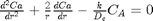A mole balance on the particle volume in spherical coordinates with a first order reaction leads to: with boundary conditions and at . We convert this equation to a system of first order ODEs by letting .

    function dYdt = ode(r,Y)

        Wa = Y(1); % molar rate of delivery of A to surface of particle
        Ca = Y(2); % concentration of A in the particle at r

        if r == 0
            dWadr = 0; % this solves the singularity at r = 0
        else
            dWadr = -2*Wa/r + k/De*Ca;
        end

        dCadr = Wa;

        dYdt = [dWadr; dCadr];
    end

Parameters for this problem

De = 0.1;   % diffusivity cm^2/s
R = 0.5;    % particle radius, cm
k = 6.4;    % rate constant (1/s)
CAs = 0.2;  % concentration of A at outer radius of particle (mol/L)

Solving the BVP

we have a condition of no flux at r=0 and Ca® = CAs, which makes this a boundary value problem. We use the shooting method here, and guess what Ca(0) is and iterate the guess to get Ca® = CAs.

Ca0 = 0.029315; % Ca(0) (mol/L) guessed to satisfy Ca(R) = CAs
Wa0 = 0;    % no flux at r=0 (mol/m^2/s)
init = [Wa0 Ca0];
rspan = [0 R];

[r Y] = ode45(@ode,rspan, init);
Ca = Y(:,2);

plot(r,Ca)
xlabel('Particle radius')
ylabel('C_A')

You can see the concentration of A inside the particle is significantly lower than outside the particle. That is because it is reacting away faster than it can diffuse into the particle. Hence, the overall reaction rate in the particle is lower than it would be without the diffusion limit.

Compute the effectiveness factor numerically

The effectiveness factor is the ratio of the actual reaction rate in the particle with diffusion limitation to the ideal rate in the particle if there was no concentration gradient:

We will evaluate this numerically from our solution.

eta_numerical = trapz(r, k*Ca*4*pi.*(r.^2))/trapz(r, k*CAs*4*pi.*(r.^2))

eta_numerical =

    0.5635

Analytical solution for a first order reaction

an analytical solution exists for this problem.

phi = R*sqrt(k/De);
eta = (3/phi^2)*(phi*coth(phi)-1)

eta =

    0.5630

Why go through the numerical solution when an analytical solution exists? The analytical solution here is only good for 1st order kinetics in a sphere. What would you do for a complicated rate law? You might be able to find some limiting conditions where the analytical equation above is relevant, and if you are lucky, they are appropriate for your problem. If not, it's a good thing you can figure this out numerically!

end

% categories: BVP
% tags: reaction engineering

Published with MATLAB® 7.13

Modeling a transient plug flow reactor

John Kitchin

Contents

function main

clear all; clc; close all

    function dCdt = method_of_lines(t,C)
        % we use vectorized operations to define the odes at each node
        % point.
        dCdt = [0; % C1 does not change with time, it is the entrance of the pfr
               -vo*diff(C)./diff(V)-k*C(2:end).^2];
    end

Problem setup

Ca0 = 2; % Entering concentration
vo = 2; % volumetric flow rate
volume = 20;  % total volume of reactor, spacetime = 10
k = 1;  % reaction rate constant

N = 100; % number of points to discretize the reactor volume on

init = zeros(N,1); % Concentration in reactor at t = 0
init(1) = Ca0; % concentration at entrance

V = linspace(0,volume,N)'; % discretized volume elements, in column form

tspan = [0 20];
[t,C] = ode15s(@method_of_lines,tspan,init);

plotting the solution

The solution contains the time dependent behavior of each node in the discretized reactor. For example, we can plot the concentration of A at the exit vs. time as:

plot(t,C(:,end))
xlabel('time')
ylabel('Concentration at exit')

You can see that around the space time, species A breaks through the end of the reactor, and rapidly rises to a steady state value.

animating the solution

It isn't really illustrative to examine only the exit concentration. We can also create an animated gif to show how the concentration of A throughout the reactor varies with time.

filename = 'transient-pfr.gif'; % file to store image in
for i=1:5:length(t) % only look at every 5th time step
    plot(V,C(i,:));
    ylim([0 2])
    xlabel('Reactor volume')
    ylabel('C_A')
    text(0.1,1.9,sprintf('t = %1.2f',t(i))); % add text annotation of time step
    frame = getframe(1);
    im = frame2im(frame); %convert frame to an image
    [imind,cm] = rgb2ind(im,256);

    % now we write out the image to the animated gif.
    if i == 1;
        imwrite(imind,cm,filename,'gif', 'Loopcount',inf);
    else
        imwrite(imind,cm,filename,'gif','WriteMode','append');
    end
end
close all; % makes sure the plot from the loop above doesn't get published

here is the animation!

You can see that the steady state behavior is reached at approximately 10 time units, which is the space time of the reactor in this example.

Add steady state solution

It is good to double check that we get the right steady state behavior. We can solve the steady state plug flow reactor problem like this:

    function dCdV = pfr(V,C)
        dCdV = 1/vo*(-k*C^2);
    end

figure; hold all
vspan = [0 20];
[V_ss Ca_ss] = ode45(@pfr,vspan,2);
plot(V_ss,Ca_ss,'k--','linewidth',2)
plot(V,C(end,:),'r') % last solution of transient part
legend 'Steady state solution' 'transient solution at t=100'

there is some minor disagreement between the final transient solution and the steady state solution. That is due to the approximation in discretizing the reactor volume. In this example we used 100 nodes. You get better agreement with a larger number of nodes, say 200 or more. Of course, it takes slightly longer to compute then, since the number of coupled odes is equal to the number of nodes.

end

% categories: PDEs
% tags: reaction engineering

Published with MATLAB® 7.13