Finding equilibrium composition by direct minimization of Gibbs free energy on mole numbers

| categories: optimization | View Comments

Finding equilibrium composition by direct minimization of Gibbs free energy on mole numbers

Finding equilibrium composition by direct minimization of Gibbs free energy on mole numbers

John Kitchin

Adapted from problem 4.5 in Cutlip and Shacham

Contents

Problem setup

Ethane and steam are fed to a steam cracker at a total pressure of 1 atm and at 1000K at a ratio of 4 mol H2O to 1 mol ethane. Estimate the equilibrium distribution of products (CH4, C2H4, C2H2, CO2, CO, O2, H2, H2O, and C2H6).

Solution method: We will construct a Gibbs energy function for the mixture, and obtain the equilibrium composition by minimization of the function subject to elemental mass balance constraints.

function main
R = 0.00198588; % kcal/mol/K
T = 1000; % K

% we store the species names in a cell array since they have different
% lengths (i.e. different number of characters in names).
species = {'CH4' 'C2H4' 'C2H2' 'CO2' 'CO' 'O2' 'H2' 'H2O' 'C2H6'};

%
% $G_^\circ for each species. These are the heats of formation for each
% species.
Gjo = [4.61 28.249 40.604 -94.61 -47.942 0 0 -46.03 26.13]; % kcal/mol

The Gibbs energy of a mixture

We start with $G=\sum\limits_j n_j \mu_j$. Recalling that we define $\mu_j = G_j^\circ + RT \ln a_j$, and in the ideal gas limit, $a_j = y_j P/P^\circ$, and that $y_j = \frac{n_j}{\sum n_j}$. Since in this problem, P = 1 atm, this leads to the function $\frac{G}{RT} = \sum\limits_{j=1}^n n_j\left(\frac{G_j^\circ}{RT} + \ln \frac{n_j}{\sum n_j}\right)$.

    function G = func(nj)
        Enj = sum(nj);
        G = sum(nj.*(Gjo/R/T + log(nj/Enj)));
    end

Linear equality constraints for atomic mass conservation

The total number of each type of atom must be the same as what entered the reactor. These form equality constraints on the equilibrium composition. We express these constraints as: $A_{eq} x = b$ where $x$ is a vector of the moles of each species present in the mixture. CH4 C2H4 C2H2 CO2 CO O2 H2 H2O C2H6

Aeq = [0   0    0    2   1  2  0  1   0       % oxygen balance
       4   4    2    0   0  0  2  2   6       % hydrogen balance
       1   2    2    1   1  0  0  0   2];     % carbon balance

% the incoming feed was 4 mol H2O and 1 mol ethane
beq = [4    % moles of oxygen atoms coming in
       14   % moles of hydrogen atoms coming in
       2];  % moles of carbon atoms coming in

Bounds on mole numbers

No mole number can be negative, so we define a lower bound of zero for each mole number. In principle there are upper bounds too, but it is unecessary to define them here.

LB = [0 0 0 0 0 0 0 0 0]; % no mole numbers less than zero

initial guess for the solver

these are the guesses suggested in the book.

x0 = [1e-3 1e-3 1e-3 0.993 1 1e-4 5.992 1 1e-3]; % initial guess

Setup minimization

fmincon does not solve this problem with the default solver, and warns you to pick another one, either 'interior-point' or 'sqp'. Both work for this problem.

options = optimset('Algorithm','sqp');
[x fval] = fmincon(@func,x0,[],[],Aeq,beq,LB,[],[],options);

for i=1:numel(x)
    fprintf('%5d%10s%10.3g\n',i,species{i},x(i))
end
Local minimum possible. Constraints satisfied.

fmincon stopped because the size of the current step is less than
the default value of the step size tolerance and constraints are 
satisfied to within the default value of the constraint tolerance.


    1       CH4    0.0664
    2      C2H4 8.88e-008
    3      C2H2 2.76e-021
    4       CO2     0.545
    5        CO      1.39
    6        O2 4.56e-021
    7        H2      5.35
    8       H2O      1.52
    9      C2H6  1.6e-007

Verify the equality constraints were met

you can see here the constraints were met.

Aeq*x'
beq
ans =

     4
    14
     2


beq =

     4
    14
     2

Results

Interestingly there is a distribution of products! That is interesting because only steam and ethane enter the reactor, but a small fraction of methane is formed! The main product is hydrogen. The stoichiometry of steam reforming is ideally $C_2H_6 + 4H_2O \rightarrow 2CO_2 + 7 H2$. Even though nearly all the ethane is consumed, we don't get the full yield of hydrogen. It appears that another equilibrium, one between CO, CO2, H2O and H2, may be limiting that, since the rest of the hydrogen is largely in the water. It is also of great importance that we have not said anything about reactions, i.e. how these products were formed. This is in stark contrast to Post 1589 where stoichiometric coefficients were necessary to perform the minimization.

Water gas shift equilibrium

The water gas shift reaction is: $CO + H_2O \rightleftharpoons CO_2 + H_2$. We can compute the Gibbs free energy of the reaction from the heats of formation of each species. Assuming these are the formation energies at 1000K, this is the reaction free energy at 1000K.

G_wgs = Gjo(4) + Gjo(7) - Gjo(5) - Gjo(8)
G_wgs =

   -0.6380

WGS equilibrium constant at 1000K

exp(-G_wgs/R/T)
ans =

    1.3789

Equilibrium constant based on mole numbers

One normally uses activities to define the equilibrium constant. Since there are the same number of moles on each side of the reaction all factors that convert mole numbers to activity, concentration or pressure cancel, so we simply consider the ratio of mole numbers here.

x(4)*x(7)/(x(5)*x(8))
ans =

    1.3789

Clearly, there is an equilibrium between these species that prevents the complete reaction of steam reforming.

Summary

This is an appealing way to minimize the Gibbs energy of a mixture. No assumptions about reactions are necessary, and the constraints are easy to identify. The Gibbs energy function is especially easy to code.

end

% categories: optimization
% tags: Thermodynamics, reaction engineering
% post_id = 1630; %delete this line to force new post;
% permaLink = http://matlab.cheme.cmu.edu/2011/12/25/finding-equilibrium-composition-by-direct-minimization-of-gibbs-free-energy-on-mole-numbers/;
Read and Post Comments

A novel way to numerically estimate the derivative of a function - complex-step derivative approximation

| categories: miscellaneous | View Comments

A novel way to numerically estimate the derivative of a function - complex-step derivative approximation

A novel way to numerically estimate the derivative of a function - complex-step derivative approximation

John Kitchin

Adapted from http://biomedicalcomputationreview.org/2/3/8.pdf and http://dl.acm.org/citation.cfm?id=838250.838251

This posts introduces a novel way to numerically estimate the derivative of a function that does not involve finite difference schemes. Finite difference schemes are approximations to derivatives that become more and more accurate as the step size goes to zero, except that as the step size approaches the limits of machine accuracy, new errors can appear in the approximated results. In the references above, a new way to compute the derivative is presented that does not rely on differences!

The new way is: $f'(x) = \rm{imag}(f(x + i\Delta x)/\Delta x)$ where the function $f$ is evaluated in imaginary space with a small $\Delta x$ in the complex plane. The derivative is miraculously equal to the imaginary part of the result in the limit of $\Delta x \rightarrow 0$!

Contents

Example 1

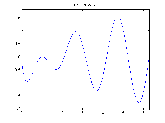
This example comes from the first link. The derivative must be evaluated using the chain rule. We compare a forward difference, central difference and complex-step derivative approximations.

f = @(x) sin(3*x)*log(x);
ezplot(f)

format long

at x = 0.7

x = 0.7;
h = 1e-7;

analytical derivative

dfdx_a = 3*cos(3*x)*log(x) + sin(3*x)/x
dfdx_a =

   1.773354106237345

finite difference

dfdx_fd = (f(x) - f(x-h))/h
dfdx_fd =

   1.773354270651062

central difference

dfdx_cd = (f(x+h)-f(x-h))/(2*h)
dfdx_cd =

   1.773354105227831

complex method

dfdx_I = imag(f(x+h*i)/h)
dfdx_I =

   1.773354106237384

compute errors

You can see the complex-step derivative approximation is several orders of magnitude more accurate than either of the finite difference methods.

dfdx_fd - dfdx_a
dfdx_cd - dfdx_a
dfdx_I - dfdx_a
ans =

    1.644137173073546e-007


ans =

   -1.009513361793779e-009


ans =

    3.952393967665557e-014

another example

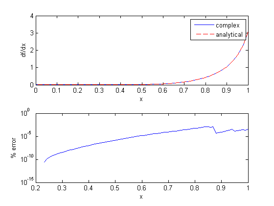
Let's use this method to verify the fundamental Theorem of Calculus, i.e. to evaluate the derivative of an integral function. Let $f(x) = \int\limits_1^{x^2} tan(t^3)dt$, and we now want to compute df/dx. Of course, this can be done analytically, but it is not trivial!
integrand = @(t) tan(t.^3);
f = @(z) quad(integrand, 0,z.^2);

Lets evaluate the derivative over a range of x-values. The quad function is not vectorized for the limits, so we have to use arrayfun to map each x-value onto a vector of dfdx. The agreement here is very good, with the largest %%error being 0.0001%% near x=1. That interestingly does not get much better with smaller h.

x = linspace(0,1);
dfdx = imag(arrayfun(f,(x+i*h))/h);
dfdx_analytical = 2*x.*tan(x.^6);

subplot(2,1,1)
plot(x,dfdx,x,dfdx_analytical,'r--')
xlabel('x')
ylabel('df/dx')
legend('complex','analytical')

subplot(2,1,2)
semilogy(x,(dfdx-dfdx_analytical)./dfdx_analytical*100)
xlabel('x')
ylabel('% error')

don't get too complacent though!

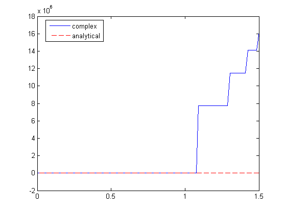
Here is an example that fails to agree!

x = linspace(0,1.5);

dfdx = imag(arrayfun(f,(x+i*h))/h);
dfdx_analytical = 2*x.*tan(x.^6);

figure
plot(x,dfdx,x,dfdx_analytical,'r--')
legend('complex','analytical','location','best')

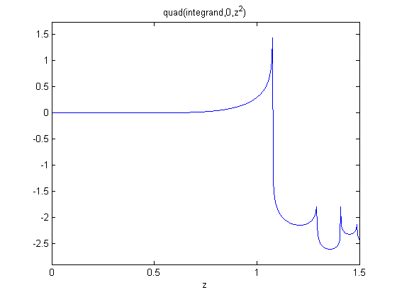
I guess the reason for the failure appears to be related to the singularity at x = 1.1. It is not clear why that causes the estimated derivative to blow up though, since it works everywhere else. It appears there is a step change at each singularity in the function.

ezplot(f,[0,1.5])

Summary

Using this simple formula $f'(x) = imag(f(x + ih)/h)$ to approximate a derivative is one of the most interesting math facts I can't believe I didn't know before this post!

% categories: Miscellaneous
Read and Post Comments

Constrained optimization

| categories: optimization | View Comments

constrained_minimization

Contents

Constrained optimization

John Kitchin

adapted from http://en.wikipedia.org/wiki/Lagrange_multipliers.

function constrained_minimization
clear all; close all

Introduction

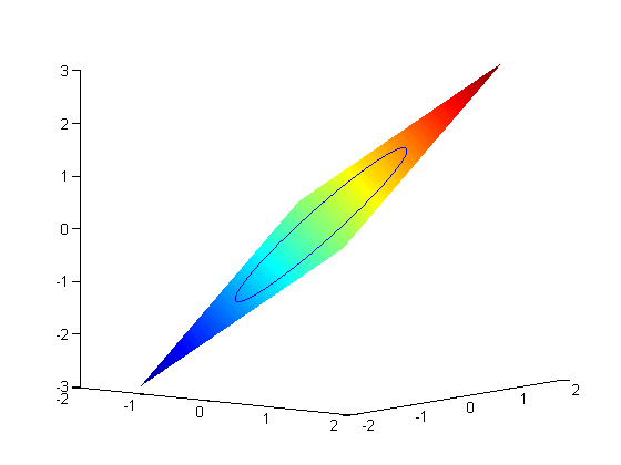
Suppose we seek to minimize the function $f(x,y)=x+y$ subject to the constraint that $x^2 + y^2 = 1$. The function we seek to maximize is an unbounded plane, while the constraint is a unit circle. In Post 1602 we setup a Lagrange multiplier approach to solving this problem. Today, we use the builtin function fmincon in Matlab to solve the same problem.
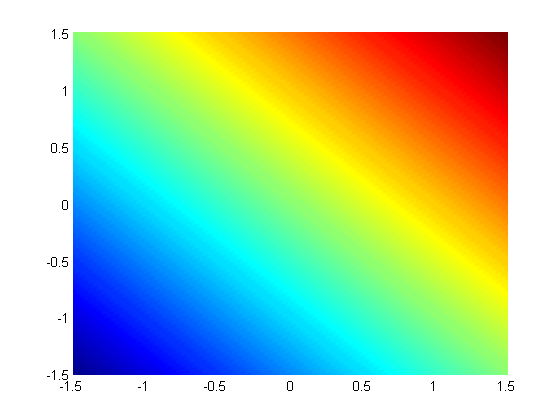
We plot these two functions here.

x = linspace(-1.5,1.5);
[X,Y] = meshgrid(x,x);
figure; hold all
surf(X,Y,X+Y);
shading interp;

now plot the circle on the plane. First we define a circle in polar

coordinates, then convert those coordinates to x,y cartesian coordinates. then we plot f(x1,y1).

theta = linspace(0,2*pi);
[x1,y1] = pol2cart(theta,1);
plot3(x1,y1,x1+y1)
view(38,8) % adjust view so it is easy to see

Construct the function to optimize and the nonlinear constraint function

the original function, provided that the constraint is met!

    function f = func(X)
        x = X(1);
        y = X(2);
        f = x + y;
    end

    function [c,ceq] = nlconstraints(X)
        % function for the nonlinear constraints.
        % We have to define two outputs for fmincon: the nonlinear
        % inequality contraints, and the equality constraints.
        %
        % C(X) <= 0
        %
        % Ceq(X) = 0

        x = X(1);
        y = X(2);
        c = [];
        ceq = x^2 + y^2 - 1;
    end

Now we solve for the problem

fmincon takes a lot of options. We define all of them here, even though in this example we do not have any linear inequality or equality constraints, and we don't define bounds on the solution. It is necessary to put these empty placeholders in the fmincon call, however, so that it knows what the nonlinear constraints are.

A   =  [];
B   =  []; % the linear inequality constraints: A*X <= B
Aeq =  [];
Beq =  []; % the linear equality constraints: Aeq*X = B
LB  =  [];
UB  =  []; % LB <= X <= UB
X0  =  [1, 1]; % initial guess

[X,FVAL,EXITFLAG,OUTPUT,LAMBDA] = fmincon(@func,X0,A,B,Aeq,Beq,LB,UB,@nlconstraints)

OUTPUT.message
plot3(X(1),X(2),FVAL,'bo','markerfacecolor','b')
Warning: The default trust-region-reflective algorithm does not
solve problems with the constraints you have specified. FMINCON
will use the active-set algorithm instead. For information on
applicable algorithms, see Choosing the Algorithm in the
documentation. 

Local minimum possible. Constraints satisfied.

fmincon stopped because the predicted change in the objective function
is less than the default value of the function tolerance and constraints 
are satisfied to within the default value of the constraint tolerance.


X =

    0.7071    0.7071


FVAL =

    1.4142


EXITFLAG =

     5


OUTPUT = 

         iterations: 5
          funcCount: 15
       lssteplength: 1
           stepsize: 5.9440e-005
          algorithm: [1x44 char]
      firstorderopt: 7.9553e-006
    constrviolation: 2.3986e-011
            message: [1x776 char]


LAMBDA = 

         lower: [2x1 double]
         upper: [2x1 double]
         eqlin: [1x0 double]
      eqnonlin: 0.7071
       ineqlin: [1x0 double]
    ineqnonlin: [1x0 double]


ans =

Local minimum possible. Constraints satisfied.

fmincon stopped because the predicted change in the objective function
is less than the default value of the function tolerance and constraints 
are satisfied to within the default value of the constraint tolerance.

Stopping criteria details:

Optimization stopped because the predicted change in the objective function,
6.856786e-010, is less than options.TolFun = 1.000000e-006, and the maximum constraint
violation, 2.398637e-011, is less than options.TolCon = 1.000000e-006.

Optimization Metric                                                 Options
abs(steplength*directional derivative) =  6.86e-010        TolFun =  1e-006 (default)
max(constraint violation) =  2.40e-011                     TolCon =  1e-006 (default)

Note the warning about the algorithm change. Matlab automatically detected that it could not use the default algorithm because of the nonlinear constraints. Matlab also automatically selected a better algorithm for you.

There is a lot of output, that mostly tells us the function worked as expected. Note that the solution above is not a global minimum. There is another solution at the bottom of the circle. Let's try another initial guess.

X0 = [-1, -1];
[X,FVAL,EXITFLAG,OUTPUT,LAMBDA] = fmincon(@func,X0,A,B,Aeq,Beq,LB,UB,@nlconstraints)
plot3(X(1),X(2),FVAL,'ro','markerfacecolor','r')
Warning: The default trust-region-reflective algorithm does not
solve problems with the constraints you have specified. FMINCON
will use the active-set algorithm instead. For information on
applicable algorithms, see Choosing the Algorithm in the
documentation. 

Local minimum found that satisfies the constraints.

Optimization completed because the objective function is non-decreasing in 
feasible directions, to within the default value of the function tolerance,
and constraints are satisfied to within the default value of the constraint tolerance.


X =

   -0.7071   -0.7071


FVAL =

   -1.4142


EXITFLAG =

     1


OUTPUT = 

         iterations: 4
          funcCount: 15
       lssteplength: 1
           stepsize: 1.5019e-006
          algorithm: [1x44 char]
      firstorderopt: 1.0880e-008
    constrviolation: 2.2982e-012
            message: [1x787 char]


LAMBDA = 

         lower: [2x1 double]
         upper: [2x1 double]
         eqlin: [1x0 double]
      eqnonlin: 0.7071
       ineqlin: [1x0 double]
    ineqnonlin: [1x0 double]

This is the global minimum (by inspection).

Summary

the built in function fmincon is more flexible than what we did in Post 1602 since it includes inequality constraints. Of course, that flexibility comes at some cost, you have to know the expected syntax for each kind of constraint. But that is easy to find out with the Matlab documentation.

end

% categories: optimization
Read and Post Comments

Using Lagrange multipliers in optimization

| categories: optimization | View Comments

lagrange_multiplier

Contents

Using Lagrange multipliers in optimization

John Kitchin

adapted from http://en.wikipedia.org/wiki/Lagrange_multipliers.

function lagrange_multiplier
clear all; close all

Introduction

Suppose we seek to maximize the function $f(x,y)=x+y$ subject to the constraint that $x^2 + y^2 = 1$. The function we seek to maximize is an unbounded plane, while the constraint is a unit circle. We plot these two functions here.

x = linspace(-1.5,1.5);
[X,Y] = meshgrid(x,x);
figure; hold all
surf(X,Y,X+Y);
shading interp;

now plot the circle on the plane. First we define a circle in polar

coordinates, then convert those coordinates to x,y cartesian coordinates. then we plot f(x1,y1).

theta = linspace(0,2*pi);
[x1,y1] = pol2cart(theta,1);
plot3(x1,y1,x1+y1)
view(38,8) % adjust view so it is easy to see

Construct the Lagrange multiplier augmented function

To find the maximum, we construct the following function: $\Lambda(x,y; \lambda) = f(x,y)+\lambda g(x,y)$ where $g(x,y) = x^2 + y^2 - 1 = 0$, which is the constraint function. Since $g(x,y)=0$, we aren't really changing the original function, provided that the constraint is met!

    function gamma = func(X)
        x = X(1);
        y = X(2);
        lambda = X(3);
        gamma = x + y + lambda*(x^2 + y^2 - 1);
    end

Finding the partial derivatives

The minima/maxima of the augmented function are located where all of the partial derivatives of the augmented function are equal to zero, i.e. $\partial \Lambda/\partial x = 0$, $\partial \Lambda/\partial y = 0$, and $\partial \Lambda/\partial \lambda = 0$. the process for solving this is usually to analytically evaluate the partial derivatives, and then solve the unconstrained resulting equations, which may be nonlinear.

Rather than perform the analytical differentiation, here we develop a way to numerically approximate the partial derivates.

    function dLambda = dfunc(X)

function to compute the partial derivatives of the function defined above at the point X. We use a central finite difference approach to compute $\partial \Lambda/\partial x_i$.

       % initialize the partial derivative vector so it has the same shape
       % as the input X
       dLambda = nan(size(X));

       h = 1e-3; % this is the step size used in the finite difference.
       for i=1:numel(X)
           dX=zeros(size(X));
           dX(i) = h;
           dLambda(i) = (func(X+dX)-func(X-dX))/(2*h);
       end
    end

Now we solve for the zeros in the partial derivatives

The function we defined above (dfunc) will equal zero at a maximum or minimum. It turns out there are two solutions to this problem, but only one of them is the maximum value. Which solution you get depends on the initial guess provided to the solver. Here we have to use some judgement to identify the maximum.

X1 = fsolve(@dfunc,[1 1 0],optimset('display','off'))
% let's check the value of the function at this solution
fval1 = func(X1)
sprintf('%f',fval1)

I don't know why the output in publish doesn't show up in the right place. sometimes that happens. The output from the cell above shows up at the end of the output for some reason.

Add solutions to the graph

plot3(X1(1),X1(2),fval1,'ro','markerfacecolor','b')

Summary

Lagrange multipliers are a useful way to solve optimization problems with equality constraints. The finite difference approach used to approximate the partial derivatives is handy in the sense that we don't have to do the calculus to get the analytical derivatives. It is only an approximation to the partial derivatives though, and could be problematic for some problems. An adaptive method to more accurately estimate the derivatives would be helpful, but could be computationally expensive. The significant advantage of the numerical derivatives is that it works no matter how many variables there are without even changing the code!

There are other approaches to solving this kind of equation in Matlab, notably the use of fmincon.

'done'
ans =

done

end

% categories: optimization
X1 =

    0.7071    0.7071   -0.7071


fval1 =

    1.4142


ans =

1.414214

Read and Post Comments

The Gibbs free energy of a reacting mixture and the equilibrium composition

| categories: optimization | View Comments

The Gibbs free energy of a reacting mixture and the equilibrium composition

The Gibbs free energy of a reacting mixture and the equilibrium composition

John Kitchin

Adapted from Chapter 3 in Rawlings and Ekerdt.

Contents

Introduction

In this post we derive the equations needed to find the equilibrium composition of a reacting mixture. We use the method of direct minimization of the Gibbs free energy of the reacting mixture.

The Gibbs free energy of a mixture is defined as $G = \sum\limits_j \mu_j n_j$ where $\mu_j$ is the chemical potential of species $j$, and it is temperature and pressure dependent, and $n_j$ is the number of moles of species $j$.

We define the chemical potential as $\mu_j = G_j^\circ + RT\ln a_j$, where $G_j^\circ$ is the Gibbs energy in a standard state, and $a_j$ is the activity of species $j$ if the pressure and temperature are not at standard state conditions.

If a reaction is occurring, then the number of moles of each species are related to each other through the reaction extent $\epsilon$ and stoichiometric coefficients: $n_j = n_{j0} + \nu_j \epsilon$. Note that the reaction extent has units of moles.

Combining these three equations and expanding the terms leads to:

$$G = \sum\limits_j n_{j0}G_j^\circ
     +\sum\limits_j \nu_j G_j^\circ \epsilon
     +RT\sum\limits_j(n_{j0} + \nu_j\epsilon)\ln a_j
$$

The first term is simply the initial Gibbs free energy that is present before any reaction begins, and it is a constant. It is difficult to evaluate, so we will move it to the left side of the equation in the next step, because it does not matter what its value is since it is a constant. The second term is related to the Gibbs free energy of reaction: $\Delta_rG = \sum\limits_j \nu_j G_j^\circ$. With these observations we rewrite the equation as:

$$G - \sum\limits_j n_{j0}G_j^\circ =
 \Delta_rG \epsilon
+RT\sum\limits_j(n_{j0} + \nu_j\epsilon)\ln a_j
$$

Now, we have an equation that allows us to compute the change in Gibbs free energy as a function of the reaction extent, initial number of moles of each species, and the activities of each species. This difference in Gibbs free energy has no natural scale, and depends on the size of the system, i.e. on $n_{j0}$. It is desirable to avoid this, so we now rescale the equation by the total initial moles present, $n_{T0}$ and define a new variable $\epsilon' = \epsilon/n_{T0}$, which is dimensionless. This leads to:

$$ \frac{G - \sum\limits_j n_{j0}G_j^\circ}{n_{T0}} =
  \Delta_rG \epsilon'
+ RT \sum\limits_j(y_{j0} + \nu_j\epsilon')\ln a_j
$$

where $y_{j0}$ is the initial mole fraction of species $j$ present. The mole fractions are intensive properties that do not depend on the system size. Finally, we need to address $a_j$. For an ideal gas, we know that $A_j = \frac{y_j P}{P^\circ}$, where the numerator is the partial pressure of species $j$ computed from the mole fraction of species $j$ times the total pressure. To get the mole fraction we note:

$$y_j = \frac{n_j}{n_T} = \frac{n_{j0} + \nu_j \epsilon}{n_{T0} +
\epsilon \sum\limits_j \nu_j}
= \frac{y_{j0} + \nu_j \epsilon'}{1 + \epsilon'\sum\limits_j \nu_j}
$$

This finally leads us to an equation that we can evaluate as a function of reaction extent:

$$ \frac{G - \sum\limits_j n_{j0}G_j^\circ}{n_{T0}} =
\widetilde{\widetilde{G}} =
\Delta_rG \epsilon'
+ RT\sum\limits_j(y_{j0} + \nu_j\epsilon')
\ln\left(\frac{y_{j0}+\nu_j\epsilon'}{1+\epsilon'\sum\limits_j\nu_j}
 \frac{P}{P^\circ}\right)
$$

we use a double tilde notation to distinguish this quantity from the quantity derived by Rawlings and Ekerdt which is further normalized by a factor of $RT$. This additional scaling makes the quantities dimensionless, and makes the quantity have a magnitude of order unity, but otherwise has no effect on the shape of the graph.

Finally, if we know the initial mole fractions, the initial total pressure, the Gibbs energy of reaction, and the stoichiometric coefficients, we can plot the scaled reacting mixture energy as a function of reaction extent. At equilibrium, this energy will be a minimum. We consider the example in Rawlings and Ekerdt where isobutane (I) reacts with 1-butene (B) to form 2,2,3-trimethylpentane (P). The reaction occurs at a total pressure of 2.5 atm at 400K, with equal molar amounts of I and B. The standard Gibbs free energy of reaction at 400K is -3.72 kcal/mol. Compute the equilibrium composition.

function main
clear all; close all

u = cmu.units;
R = 8.314*u.J/u.mol/u.K;
P = 2.5*u.atm;
Po = 1*u.atm; % standard state pressure
T = 400*u.K;

Grxn = -3.72*u.kcal/u.mol; %reaction free energy at 400K
yi0 = 0.5; yb0 = 0.5; yp0 = 0.0; % initial mole fractions

yj0 = [yi0 yb0 yp0];
nu_j = [-1 -1 1]; % stoichiometric coefficients

Define a function for $\frac{G - \sum\limits_j n_{j0}G_j^\circ}{n_{T0}}$

We will call this difference Gwigglewiggle.

    function diffG = Gfunc(extentp)
        diffG = Grxn*extentp;

        sum_nu_j = sum(nu_j);
        for i = 1:length(yj0)
            x1 = yj0(i) + nu_j(i)*extentp;
            x2 = x1./(1+extentp*sum_nu_j);
            diffG = diffG + R*T*x1.*log(x2*P/Po);
        end
    end

Plot function

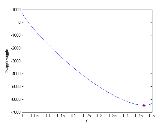
There are bounds on how large $\epsilon'$ can be. Recall that $n_j = n_{j0} + \nu_j \epsilon$, and that $n_j \ge 0$. Thus, $\epsilon_{max} = -n_{j0}/\nu_j$, and the maximum value that $\epsilon'$ can have is therefore $-y_{j0}/\nu_j$ where $y_{j0}>0$. When there are multiple species, you need the smallest $epsilon'_{max}$ to avoid getting negative mole numbers.
epsilonp_max = min(-yj0(yj0>0)./nu_j(yj0>0))
epsilonp = linspace(0,epsilonp_max,1000);
plot(epsilonp,Gfunc(epsilonp))
xlabel('\epsilon''')
ylabel('Gwigglewiggle')
epsilonp_max =

    0.5000

Find extent that minimizes Gwigglewiggle

fminbnd is not defined for the units class, so we wrap the function in a function handle that makes it output a double. Alternatively, we could make the function fully dimensionless. We save that for a later post.

f = @(x) double(Gfunc(x))
epsilonp_eq = fminbnd(f,0,epsilonp_max)

hold on
plot(epsilonp_eq,Gfunc(epsilonp_eq),'ro')
f = 

    @(x)double(Gfunc(x))


epsilonp_eq =

    0.4696

Compute equilibrium mole fractions

yi = (yi0 + nu_j(1)*epsilonp_eq)/(1 + epsilonp_eq*sum(nu_j))
yb = (yb0 + nu_j(2)*epsilonp_eq)/(1 + epsilonp_eq*sum(nu_j))
yp = (yp0 + nu_j(3)*epsilonp_eq)/(1 + epsilonp_eq*sum(nu_j))
yi =

    0.0572


yb =

    0.0572


yp =

    0.8855

alternative way to compute mole fractions

y_j = (yj0 + nu_j*epsilonp_eq)/(1 + epsilonp_eq*sum(nu_j))
y_j =

    0.0572    0.0572    0.8855

Check for consistency with the equilibrium constant

K = exp(-Grxn/R/T)
K =

  108.1300

$K = \frac{a_P}{a_I a_B} = \frac{y_p P/P^\circ}{y_i P/P^\circ y_b P/P^\circ} = \frac{y_P}{y_i y_b}\frac{P^\circ}{P}$.

yp/(yi*yb)*Po/P
ans =

  108.0702

an alternative form of the equilibrium constant

We can express the equilibrium constant like this :$K = \prod\limits_j a_j^{\nu_j}$, and compute it with a single command.

prod((y_j*P/Po).^nu_j)
ans =

  108.0702

These results are very close, and only disagree because of the default tolerance used in identifying the minimum of our function. you could tighten the tolerances by setting options to the fminbnd function.

Summary

In this post we derived an equation for the Gibbs free energy of a reacting mixture and used it to find the equilibrium composition. In future posts we will examine some alternate forms of the equations that may be more useful in some circumstances.

end

% categories: optimization
% tags: thermodynamics, reaction engineering
Read and Post Comments

« Previous Page -- Next Page »