Matlab in Chemical Engineering at CMU

Contents

Using Lagrange multipliers in optimization

John Kitchin

adapted from http://en.wikipedia.org/wiki/Lagrange_multipliers.

function lagrange_multiplier

clear all; close all

Introduction

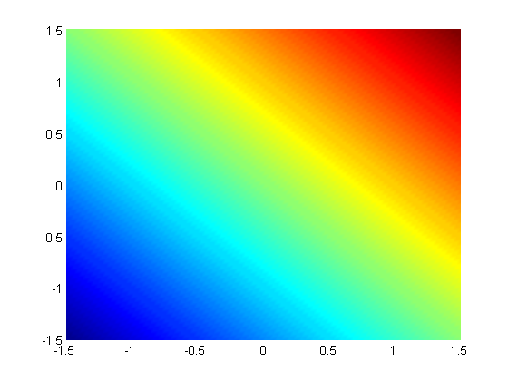
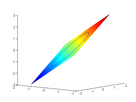
Suppose we seek to maximize the function subject to the constraint that . The function we seek to maximize is an unbounded plane, while the constraint is a unit circle. We plot these two functions here.

x = linspace(-1.5,1.5);
[X,Y] = meshgrid(x,x);
figure; hold all
surf(X,Y,X+Y);
shading interp;

now plot the circle on the plane. First we define a circle in polar

coordinates, then convert those coordinates to x,y cartesian coordinates. then we plot f(x1,y1).

theta = linspace(0,2*pi);
[x1,y1] = pol2cart(theta,1);
plot3(x1,y1,x1+y1)
view(38,8) % adjust view so it is easy to see

Construct the Lagrange multiplier augmented function

To find the maximum, we construct the following function: where , which is the constraint function. Since , we aren't really changing the original function, provided that the constraint is met!

    function gamma = func(X)
        x = X(1);
        y = X(2);
        lambda = X(3);
        gamma = x + y + lambda*(x^2 + y^2 - 1);
    end

Finding the partial derivatives

The minima/maxima of the augmented function are located where all of the partial derivatives of the augmented function are equal to zero, i.e. , , and . the process for solving this is usually to analytically evaluate the partial derivatives, and then solve the unconstrained resulting equations, which may be nonlinear.

Rather than perform the analytical differentiation, here we develop a way to numerically approximate the partial derivates.

    function dLambda = dfunc(X)

function to compute the partial derivatives of the function defined above at the point X. We use a central finite difference approach to compute .

       % initialize the partial derivative vector so it has the same shape
       % as the input X
       dLambda = nan(size(X));

       h = 1e-3; % this is the step size used in the finite difference.
       for i=1:numel(X)
           dX=zeros(size(X));
           dX(i) = h;
           dLambda(i) = (func(X+dX)-func(X-dX))/(2*h);
       end

    end

Now we solve for the zeros in the partial derivatives

The function we defined above (dfunc) will equal zero at a maximum or minimum. It turns out there are two solutions to this problem, but only one of them is the maximum value. Which solution you get depends on the initial guess provided to the solver. Here we have to use some judgement to identify the maximum.

X1 = fsolve(@dfunc,[1 1 0],optimset('display','off'))
% let's check the value of the function at this solution
fval1 = func(X1)
sprintf('%f',fval1)

I don't know why the output in publish doesn't show up in the right place. sometimes that happens. The output from the cell above shows up at the end of the output for some reason.

Add solutions to the graph

plot3(X1(1),X1(2),fval1,'ro','markerfacecolor','b')

Summary

Lagrange multipliers are a useful way to solve optimization problems with equality constraints. The finite difference approach used to approximate the partial derivatives is handy in the sense that we don't have to do the calculus to get the analytical derivatives. It is only an approximation to the partial derivatives though, and could be problematic for some problems. An adaptive method to more accurately estimate the derivatives would be helpful, but could be computationally expensive. The significant advantage of the numerical derivatives is that it works no matter how many variables there are without even changing the code!

There are other approaches to solving this kind of equation in Matlab, notably the use of fmincon.

'done'

ans =

done

end

% categories: optimization

X1 =

    0.7071    0.7071   -0.7071


fval1 =

    1.4142


ans =

1.414214

Published with MATLAB® 7.12