The Gibbs free energy of a reacting mixture and the equilibrium composition
December 20, 2011 at 05:25 PM | categories: optimization | View Comments
The Gibbs free energy of a reacting mixture and the equilibrium composition
John Kitchin
Adapted from Chapter 3 in Rawlings and Ekerdt.
Contents

Introduction
In this post we derive the equations needed to find the equilibrium composition of a reacting mixture. We use the method of direct minimization of the Gibbs free energy of the reacting mixture.
The Gibbs free energy of a mixture is defined as  where
where  is the chemical potential of species
  , and it is temperature and pressure dependent, and
  is the number of moles of species .
We define the chemical potential as  , where
  is the Gibbs energy in a standard state, and
  is the activity of species if the pressure and temperature are not at standard state conditions.
If a reaction is occurring, then the number of moles of each species are related to each other through the reaction extent  and stoichiometric coefficients:
  . Note that the reaction extent has units of moles.
Combining these three equations and expanding the terms leads to:
The first term is simply the initial Gibbs free energy that is present before any reaction begins, and it is a constant. It is difficult to evaluate, so we will move it to the left side of the equation in the next step, because it does not matter what its value is since it is a constant. The second term is related to the Gibbs free energy of reaction:  . With these observations we rewrite the equation as:
Now, we have an equation that allows us to compute the change in Gibbs free energy as a function of the reaction extent, initial number of moles of each species, and the activities of each species. This difference in Gibbs free energy has no natural scale, and depends on the size of the system, i.e. on  . It is desirable to avoid this, so we now rescale the equation by the total initial moles present,
  and define a new variable
  , which is dimensionless. This leads to:
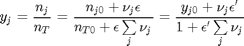
where  is the initial mole fraction of species present. The mole fractions are intensive properties that do not depend on the system size. Finally, we need to address . For an ideal gas, we know that
  , where the numerator is the partial pressure of species computed from the mole fraction of species times the total pressure. To get the mole fraction we note:
This finally leads us to an equation that we can evaluate as a function of reaction extent:
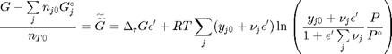
we use a double tilde notation to distinguish this quantity from the quantity derived by Rawlings and Ekerdt which is further normalized by a factor of  . This additional scaling makes the quantities dimensionless, and makes the quantity have a magnitude of order unity, but otherwise has no effect on the shape of the graph.
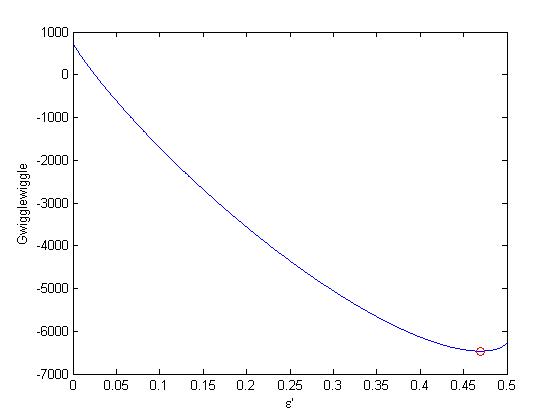
Finally, if we know the initial mole fractions, the initial total pressure, the Gibbs energy of reaction, and the stoichiometric coefficients, we can plot the scaled reacting mixture energy as a function of reaction extent. At equilibrium, this energy will be a minimum. We consider the example in Rawlings and Ekerdt where isobutane (I) reacts with 1-butene (B) to form 2,2,3-trimethylpentane (P). The reaction occurs at a total pressure of 2.5 atm at 400K, with equal molar amounts of I and B. The standard Gibbs free energy of reaction at 400K is -3.72 kcal/mol. Compute the equilibrium composition.
function main
clear all; close all

u = cmu.units;
R = 8.314*u.J/u.mol/u.K;
P = 2.5*u.atm;
Po = 1*u.atm; % standard state pressure
T = 400*u.K;

Grxn = -3.72*u.kcal/u.mol; %reaction free energy at 400K
yi0 = 0.5; yb0 = 0.5; yp0 = 0.0; % initial mole fractions

yj0 = [yi0 yb0 yp0];
nu_j = [-1 -1 1]; % stoichiometric coefficients
Define a function for 
We will call this difference Gwigglewiggle.
    function diffG = Gfunc(extentp)
        diffG = Grxn*extentp;

        sum_nu_j = sum(nu_j);
        for i = 1:length(yj0)
            x1 = yj0(i) + nu_j(i)*extentp;
            x2 = x1./(1+extentp*sum_nu_j);
            diffG = diffG + R*T*x1.*log(x2*P/Po);
        end
    end
Plot function
There are bounds on how large  can be. Recall that
  , and that
  . Thus,
  , and the maximum value that can have is therefore
  where
where  . When there are multiple species, you need the smallest
  to avoid getting negative mole numbers.
epsilonp_max = min(-yj0(yj0>0)./nu_j(yj0>0))
epsilonp = linspace(0,epsilonp_max,1000);
plot(epsilonp,Gfunc(epsilonp))
xlabel('\epsilon''')
ylabel('Gwigglewiggle')
epsilonp_max =

    0.5000

Find extent that minimizes Gwigglewiggle
fminbnd is not defined for the units class, so we wrap the function in a function handle that makes it output a double. Alternatively, we could make the function fully dimensionless. We save that for a later post.
f = @(x) double(Gfunc(x))
epsilonp_eq = fminbnd(f,0,epsilonp_max)

hold on
plot(epsilonp_eq,Gfunc(epsilonp_eq),'ro')
f =

    @(x)double(Gfunc(x))


epsilonp_eq =

    0.4696
Compute equilibrium mole fractions
yi = (yi0 + nu_j(1)*epsilonp_eq)/(1 + epsilonp_eq*sum(nu_j))
yb = (yb0 + nu_j(2)*epsilonp_eq)/(1 + epsilonp_eq*sum(nu_j))
yp = (yp0 + nu_j(3)*epsilonp_eq)/(1 + epsilonp_eq*sum(nu_j))
yi =

    0.0572


yb =

    0.0572


yp =

    0.8855
alternative way to compute mole fractions
y_j = (yj0 + nu_j*epsilonp_eq)/(1 + epsilonp_eq*sum(nu_j))
y_j =

    0.0572    0.0572    0.8855
Check for consistency with the equilibrium constant
K = exp(-Grxn/R/T)
K =

  108.1300
 .
.
yp/(yi*yb)*Po/P
ans =

  108.0702
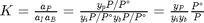
an alternative form of the equilibrium constant
We can express the equilibrium constant like this :$K = \prod\limits_j a_j^{\nu_j}$, and compute it with a single command.
prod((y_j*P/Po).^nu_j)
ans =

  108.0702
These results are very close, and only disagree because of the default tolerance used in identifying the minimum of our function. you could tighten the tolerances by setting options to the fminbnd function.
Summary
In this post we derived an equation for the Gibbs free energy of a reacting mixture and used it to find the equilibrium composition. In future posts we will examine some alternate forms of the equations that may be more useful in some circumstances.
end

% categories: optimization
% tags: thermodynamics, reaction engineering