Solving Bessel's Equation numerically

| categories: odes | View Comments

Solving Bessel's Equation numerically

Solving Bessel's Equation numerically

Reference Ch 5.5 Kreysig, Advanced Engineering Mathematics, 9th ed.

Bessel's equation $x^2 y'' + x y' + (x^2 - \nu^2)y=0$ comes up often in engineering problems such as heat transfer. The solutions to this equation are the Bessel functions. To solve this equation numerically, we must convert it to a system of first order ODEs. This can be done by letting $z = y'$ and $z' = y''$ and performing the change of variables:

$$ y' = z$$

$$ z' = \frac{1}{x^2}(-x z - (x^2 - \nu^2) y$$

if we take the case where $\nu = 0$, the solution is known to be the Bessel function $J_0(x)$, which is represented in Matlab as besselj(0,x). The initial conditions for this problem are: $y(0) = 1$ and $y'(0)=0$.

function bessel_ode
clear all; close all; clc;
% define the initial conditions
y0 = 1;
z0 = 0;
Y0 = [y0 z0];

There is a problem with our system of ODEs at x=0. Because of the $1/x^2$ term, the ODEs are not defined at x=0.

fbessel(0,Y0)
ans =

     0
   NaN

if we start very close to zero instead, we avoid the problem

fbessel(1e-15,Y0)
ans =

     0
    -1

xspan = [1e-15 10];
[x,Y] = ode45(@fbessel, xspan, Y0);

figure
hold on
plot(x,Y(:,1),'b-');
plot(x,besselj(0,x),'r--')
legend 'Numerical solution' 'analytical J_0(x)'

You can see the numerical and analytical solutions overlap, indicating they are the same.

'done'
ans =

done

function dYdx = fbessel(x,Y)
% definition of the Bessel equation as a system of first order ODEs
nu = 0;

y = Y(1);
z = Y(2);

dydx = z;
dzdx = 1/x^2*(-x*z - (x^2 - nu^2)*y);

dYdx = [dydx; dzdx];

% categories: ODEs
% tags: math
% post_id = 763; %delete this line to force new post;
Read and Post Comments

Manipulating excel with Matlab

| categories: file io | View Comments

Manipulating excel with Matlab

Manipulating excel with Matlab

John Kitchin

Sometimes there is data in an excel sheet that you want to read in, or you may want to write data to a spreadsheet. If you have a sophisticated analysis done in excel, but you want to do some analysis in Matlab, you might want to write data to the worksheet, and then read out the results.

Contents

Example setup

in our spreadsheet ( download example.xlsx ), cell B1 contains a value, and cell B2 contains $B1^2 - 1$. We can read each cell. We can also write a value to B1, and then read B2 to get the value squared. finally, we will create a function that uses Excel to perform the calculation of squaring a number, and use fsolve to minimize the function.

It is a simple example to illustrate a usage. A more realistic example might be an excel sheet where you have a complex design sheet that computes the cost of a unit operation based on properties such as volume, flow rate, etc... and you want to use Matlab to minimize the cost, but Excel to compute the cost. This is not speedy, and you may find it necessary to eventually code the whole analysis in Matlab.

function main

examples of reading

xlsread('example.xlsx','sheet1','b1')
xlsread('example.xlsx','sheet1','b2')

xlswrite('example.xlsx',4,'sheet1','b1')
ans =

     3


ans =

     8

xlsread('example.xlsx','sheet1','b1')
xlsread('example.xlsx','sheet1','b2')
% you can see we did set the value of b1 as we said, and the value of b2 is
% updated also.
ans =

     4


ans =

    15

Find roots

there are two solutions, $\pm 1$. We try guesses above and below each one.

positive root

fsolve(@f,2)
fsolve(@f,0.8)
Equation solved.

fsolve completed because the vector of function values is near zero
as measured by the default value of the function tolerance, and
the problem appears regular as measured by the gradient.


ans =

    1.0000


Equation solved.

fsolve completed because the vector of function values is near zero
as measured by the default value of the function tolerance, and
the problem appears regular as measured by the gradient.


ans =

    1.0000

negative root

fsolve(@f,-2)
fsolve(@f,-0.8)
% note it is not fast to solve this!
Equation solved.

fsolve completed because the vector of function values is near zero
as measured by the default value of the function tolerance, and
the problem appears regular as measured by the gradient.


ans =

   -1.0000


Equation solved.

fsolve completed because the vector of function values is near zero
as measured by the default value of the function tolerance, and
the problem appears regular as measured by the gradient.


ans =

   -1.0000

make a plot

x = linspace(-2,2,10);
y = arrayfun(@f,x); %this maps the function f onto the vector x

plot(x,y)
% note that this is also pretty slow.
function y = f(x)
xlswrite('example.xlsx',x,'sheet1','b1');
y = xlsread('example.xlsx','sheet1','b2');

% categories: File IO

% post_id = 739; %delete this line to force new post;
Read and Post Comments

Reading in delimited text files

| categories: basic matlab | View Comments

Reading in delimited text files

Reading in delimited text files

sometimes you will get data in a delimited text file format, .e.g. separated by commas or tabs. Matlab can read these in easily. Suppose we have a file containing this data ( download testdata.txt ):

1   3
3   4
5   6
4   8
% this is how you read it in.
A = textread('testdata.txt')

x = A(:,1);
y = A(:,2);

% you can do what ever you want with this data now. Plot it, integrate it,
% etc...

% categories: Basic matlab
% post_id = 722; %delete this line to force new post;
A =

     1     3
     3     4
     5     6
     4     8

Read and Post Comments

first order reversible reaction in batch reactor

| categories: odes | View Comments

first order reversible reaction in batch reactor

first order reversible reaction in batch reactor

John Kitchin

Contents

Problem statement

$A \rightleftharpoons B$

forward rate law: $-r_a = k_1 C_A$

backward rate law: $-r_b = k_{-1} C_B$

this example illustrates a set of coupled first order ODES

function main
clc; clear all; close all;

u = cmu.units; %note that using units makes this m-file run pretty slowly
tspan = [0 5]*u.min;
init = [1 0]*u.mol/u.L;

[t,C] = ode45(@myode,tspan,init);

plot the solution

plot(t/u.min,C/(u.mol/u.L))
xlabel('Time (min)')
ylabel('Concentration (mol/L)')
legend C_A C_B

you need this to make the plot appear in the right place above when published. It appears you need a final cell with an output to avoid having the plot showup at the end of the published document.

disp('end')
end
function dCdt = myode(t,C)
% ra = -k1*Ca
% rb = -k_1*Cb
% net rate for production of A:  ra - rb
% net rate for production of B: -ra + rb
u = cmu.units;
k1 = 1/u.min;
k_1 = 0.5/u.min;

Ca = C(1);
Cb = C(2);

ra = -k1*Ca; rb = -k_1*Cb;

dCadt = ra - rb;
dCbdt = -ra + rb;

dCdt = [dCadt; dCbdt];

% categories: ODEs
% tags: reaction engineering


% post_id = 706; %delete this line to force new post;
Read and Post Comments

Using cmu.units in Matlab for basic calculations

| categories: uncategorized | View Comments

unit_tutorials

Contents

Using cmu.units in Matlab for basic calculations

note you need to install the +cmu package for this to work.

clear all; clc; close all;

Load the units package

units is a new type of object in Matlab that stores the units, enforces proper unit algebra and works with most mathematical operations in Matlab. You load the units package into a variable; by convention: u the default set of base units are the SI units.

u = cmu.units;

Simple unit algebra

the basics of unit algebra are that like units can be added and subtracted. Unlike units can be multiplied and divided. when you assign a unit to a number, it is automatically converted into the base units.

5*u.kg % a mass
5*u.lb % another mass
6*u.m/u.s  % a velocity

1*u.m + 10*u.cm % this is ok, 1.1 m
% 1*u.m + 1*u.s  % this is not ok
5*kg
2.26796*kg
6*m/s
1.1*m

Temperature is a little special

most unit conversions are simple multiplications. Temperature conversions involve multiplication and an offset; e.g. F = C*9/5 + 32;

T = 298*u.K    % Kelvin is an absolute scale
Tf = 400*u.R   % Rankine is an absolute scale
T1 = u.degC(100) % this is 100 degC, and T1 is in Kelvin
T2 = u.degF(212) % this is 212 degF, and T2 is in Kelvin

% convert 32 degF to degC
u.degF2C(32)  %no units on the output
u.degC2F(100) %no units on the output
298*K
222.222*K
373.15*K
373.15*K

ans =

     0


ans =

   212

displaying units

a unit object has an "as" function that can display the unit in various forms

a = 1*u.kg;
a.as(u.lb)

% to do an actual conversion, you divide the unit by the units you want to
% convert to.
sprintf('%1.2f = %1.2f lb',a,a/u.lb)
ans =

2.205*lb


ans =

1.00 kg = 2.20 lb

Load the cmu.constants package

The gas constant, speed of light, etc... are stored in this package

clear all; u = cmu.units;
c = cmu.constants;
c.R  %the gas constant%% variations of the gas constant
c.R.as(u.J/u.mol/u.K)
c.R.as(u.J/(u.mol*u.K))
c.R.as(u.cal/u.mol/u.K)
c.R.as(u.dm^3*u.atm/u.mol/u.K)
c.R.as(u.BTU/u.lbmol/u.R)
c.R.as(u.ft^3*u.atm/(u.lbmol*u.R))
8.31447*m^2/s^2*kg/K/mol

ans =

8.314*J/mol/K


ans =

8.314*J/(mol*K)


ans =

1.986*cal/mol/K


ans =

0.082*dm^3*atm/mol/K


ans =

1.986*BTU/lbmol/R


ans =

0.730*ft^3*atm/(lbmol*R)

Arrays of units

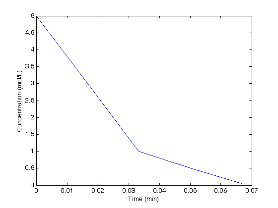
t = [0 1 2 3 4]*u.s;
C = [5 3 1 0.5 0.05]*u.mol/u.L; % note these concentrations are stored
                                % internally as mol/m^3 because those are
                                % the base SI units

% we can change the units in a plot by converting them to the units we want
plot(t/u.min,C/(u.mol/u.L))
xlabel('Time (min)')
ylabel('Concentration (mol/L)')

units with Matlab functions

Many functions in Matlab such as ode45, ode15s, fzero, fsolve, min, max, etc... work with units. This works because we have overloaded these functions to work with units. Not all functions are overloaded though, so be careful! If you find you have lost the units, it means you used a function that was not overloaded. Please let us know about it!

functions that do not work with units

functions that require dimensionless arguments (e.g. trig functions, exp, log, etc...) will usually fail if you pass a unit in. You must divide the arguments by the appropriate units to make them dimensionless

a = 5*u.mol;
sin(a/u.mol)
ans =

   -0.9589

Alternative base units

you can specify 'SI', 'CGS' or 'American' as the base units SI/MKS: {'m','s','kg', 'K', 'mol','coul'} CGS: {'cm','s','gm','K', 'mol','coul'} American: {'in','s','lb','R', 'mol','coul'

u = cmu.units('American');
a = 2*u.ft
a.as(u.m)

% you can also specify which units are your base. Note the order of base
% units must be: length, time, mass, temperature, charge, mol
% and all of them must be specified.
u = cmu.unit.units('mm','min','ton','R','coul','mol');
a = u.cm
a.as(u.m)
24*in

ans =

0.610*m

10*mm

ans =

0.010*m

simplified units

there may be times when you need units conversion, but you only want simple numbers and not unit objects, e.g. because some Matlab function doesn't handle units. You can load the simple_units structure to get a set of conversion factors. Unit algebra is not used and units are kept track of, so you have to know what the units are.

u = cmu.unit.simple_units;
a = 1*u.kg
a/u.lb
a/u.min

% tags: units, +cmu
a =

    0.0011


ans =

    2.2046


ans =

    0.0011

Read and Post Comments

« Previous Page -- Next Page »