ODEs with discontinuous forcing functions

John Kitchin  

Contents

Problem statement

Adapted from http://archives.math.utk.edu/ICTCM/VOL18/S046/paper.pdf A mixing tank initially contains 300 g of salt mixed into 1000 L of water. at t=0 min, a solution of 4 g/L salt enters the tank at 6 L/min. at t=10 min, the solution is changed to 2 g/L salt, still entering at 6 L/min. The tank is well stirred, and the tank solution leaves at a rate of 6 L/min. Plot the concentration of salt (g/L) in the tank as a function of time.

Solution

A mass balance on the salt in the tank leads to this differential equation: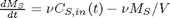 with the initial condition that 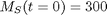. The wrinkle is that

function main

tspan = [0,15]; % min
Mo = 300; % gm salt
[t,M] = ode45(@mass_balance,tspan,Mo);

V = 1000; % L
plot(t,M/V,'b.-')
xlabel('Time (min)')
ylabel('Salt concentration (g/L)')

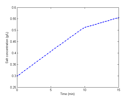You can see the discontinuity in the salt concentration at 10 minutes due to the discontinous change in the entering salt concentration.

'done'

ans =

done

discontinuous feed concentration function

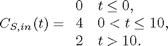
function Cs = Cs_in(t)

if t < 0
    Cs = 0; % g/L
elseif t > 0 && t <= 10
    Cs = 4; % g/L
else
    Cs = 2; % g/L
end

function dMsdt = mass_balance(t,Ms)

V = 1000; % L
nu = 6;   % L/min
dMsdt = nu*Cs_in(t) - nu*Ms/V;

% categories: ODEs

Published with MATLAB® 7.12

Solving an ode for a specific solution value

John Kitchin 8/31/2011

The analytical solution to an ODE is a function, which can be solved to get a particular value, e.g. if the solution to an ODE is y(x) = exp(x), you can solve the solution to find the value of x that makes . In a numerical solution to an ODE we get a vector of independent variable values, and the corresponding function values at those values. To solve for a particular function value we need a different approach. This post will show one way to do that in Matlab.

Contents

The problem

given that the concentration of a species A in a constant volume, batch reactor obeys this differential equation with the initial condition 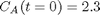mol/L and L/mol/s, compute the time it takes for to be reduced to 1 mol/L.

Solution

we will use Matlab to integrate the ODE to obtain the solution, and then use the deval command in conjuction with fsolve to get the numerical solution we are after.

clear all; close all; clc

k = 0.23;
Cao = 2.3;
dCadt = @(t,Ca) -k*Ca^2;
tspan = [0 10];
sol = ode45(dCadt,tspan,Cao)
% sol here is a struct with fields corresponding to the solution and other
% outputs of the solver.

sol = 

     solver: 'ode45'
    extdata: [1x1 struct]
          x: [1x12 double]
          y: [1x12 double]
      stats: [1x1 struct]
      idata: [1x1 struct]

We need to make sure the solution vector from the ode solver contains the answer we need

plot(sol.x,sol.y)
xlabel('Time (s)')
ylabel('C_A (mol/L)')
% the concentration of A is at approximately t=3

We can make a function Ca(t) using the solution from the ode solver and the deval command, which evaluates the ODE solution at a new value of t.

Ca = @(t) deval(sol,t);

% now we create a function for fsolve to work on. remember this function is
% equal to zero at the solution.
tguess = 3;
f = @(t) 1 - Ca(t) ;
t_solution = fsolve(f,tguess)

Ca(t_solution) % this should be 1.0

sprintf('C_A = 1 mol/L at a time of %1.2f seconds.',t_solution)

Equation solved.

fsolve completed because the vector of function values is near zero
as measured by the default value of the function tolerance, and
the problem appears regular as measured by the gradient.




t_solution =

    2.4598


ans =

    1.0000


ans =

C_A = 1 mol/L at a time of 2.46 seconds.

A related post is Post 954 on solving integral equations.

'done'

% categories: ODEs
% tags: reaction engineering
% post_id = 968; %delete this line to force new post;

ans =

done

Published with MATLAB® 7.12

Solving integral equations

John Kitchin

Contents

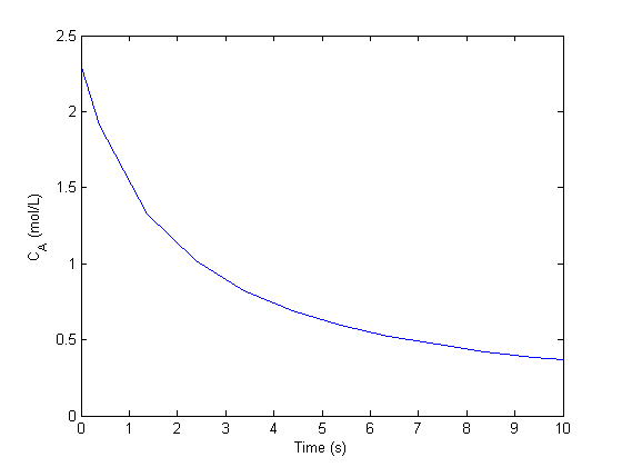
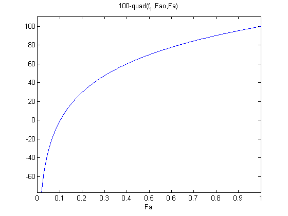
Occasionally we have integral equations we need to solve in engineering problems, for example, the volume of plug flow reactor can be defined by this equation: where is the rate law. Suppose we know the reactor volume is 100 L, the inlet molar flow of A is 1 mol/L, the volumetric flow is 10 L/min, and , with 1/min. What is the exit molar flow rate? We need to solve the following equation:

k = 0.23;
nu = 10;
Fao = 1;

We start by creating a function handle that describes the integrand. We can use this function in the quad command to evaluate the integral.

f1 = @(Fa) -1./(k*Fa/nu);

Now we create a second function handle that defines the equation to solve. We use the integrand function handle above in the quad command to evaluate the integral

f2 = @(Fa) 100 - quad(f1,Fao,Fa);

plot f2 to get an idea of where the solution is.

the maximum that Fa can be is Fao, and the minimum is zero. From the graph you can see the solution is at approximately Fa = 0.1.

ezplot(f2,0,Fao)

Warning: Function failed to evaluate on array inputs; vectorizing the function may
speed up its evaluation and avoid the need to loop over array elements. 

Get the solution

Fa_guess = 0.1;
Fa_exit = fsolve(f2, Fa_guess);

Ca_exit = Fa_exit/nu;
sprintf('The exit concentration is %1.2f mol/L',Ca_exit)

Equation solved.

fsolve completed because the vector of function values is near zero
as measured by the default value of the function tolerance, and
the problem appears regular as measured by the gradient.




ans =

The exit concentration is 0.01 mol/L

% categories: nonlinear algebra
% tags: reaction engineering
% post_id = 954; %delete this line to force new post;

Published with MATLAB® 7.12

Contents

Nonlinear curve fitting with parameter confidence intervals

John Kitchin

clear all; close all; clc

raw data to fit

x = [0.5 0.387 0.24 0.136 0.04 0.011];
y = [1.255 1.25 1.189 1.124 0.783 0.402];

plot the data

you should usually plot your data to get a feel for how it looks.

plot(x,y,'ko')
xlabel('x')
ylabel('y')

nonlinear fitting

fit this nonlinear model y = Ax/(B+x) to the data. I use a function handle here, but I think it is cleaner and easier to read with a subfunction. here pars(1) = A, and pars(2) = B

f = @(pars,x) pars(1)*x./(pars(2)+x);

parguess = [ 1.3 0.03]; % nonlinear fits need initial guesses
[pars, resid, J] = nlinfit(x,y,f,parguess)

pars =

    1.3275    0.0265


resid =

   -0.0058    0.0074   -0.0067    0.0127   -0.0160    0.0122


J =

    0.9497   -2.3949
    0.9360   -3.0053
    0.9007   -4.4873
    0.8371   -6.8404
    0.6019  -12.0216
    0.2936  -10.4056

get the confidence interval for each parameter

the nlparci command estimates confidence intervals. The first row of the output is parameter 1, second row parameter 2, ...

alpha = 0.05; % this is for 95% confidence intervals
pars_ci = nlparci(pars,resid,'jacobian',J,'alpha',alpha)
sprintf('A is in the range of [%1.2f %1.2f] at the 95%% confidence level',pars_ci(1,:))
sprintf('B is in the range of [%1.2f %1.2f] at the 95%% confidence level',pars_ci(2,:))

pars_ci =

    1.3005    1.3545
    0.0236    0.0293


ans =

A is in the range of [1.30 1.35] at the 95% confidence level


ans =

B is in the range of [0.02 0.03] at the 95% confidence level

hold all
xfit = linspace(0.5, 0.011);
plot(xfit,f(pars,xfit),'DisplayName','fitted model')
legend show

summary

The fit looks reasonable, and the confidence intervals are "tight" and do not include zero, suggesting the parameters are significant.

% categories: data analysis

Published with MATLAB® 7.12

Linear regression with confidence intervals.

Fit a fourth order polynomial to this data and determine the confidence interval for each parameter. Data from example 5-1 in Fogler, Elements of Chemical Reaction Engineering

Contents

data to fit

note the transpose so these are column vectors

t = [0 50 100 150 200 250 300]';
Ca = [50 38 30.6 25.6 22.2 19.5 17.4]'*1e-3;

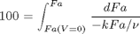
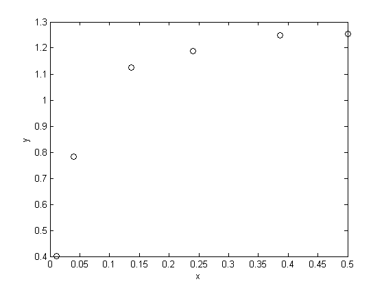
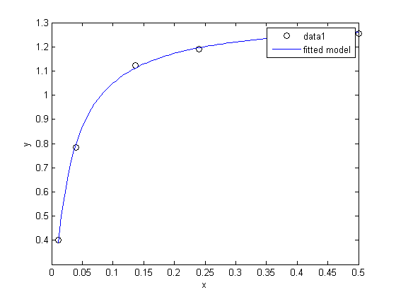
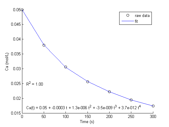
We want the equation fit to the data in the least squares sense. We can write this in a linear algebra form as: T*b = Ca where T is a matrix of columns [1 t t^2 t^3 t^4], and b is a column vector of [b0 b1 b2 b3 b4]'. We want to solve for the b vector.

T = [ones(size(t)) t t.^2 t.^3 t.^4];

% we use the :command:`regress` to solve for b
alpha = 0.05 % confidence interval is 100*(1 - alpha)
[b,bint] = regress(Ca,X, alpha)
% b is the solution to our equation
% bint is the 95% confidence interval for each parameter

% the numbers are a little small to see with the default format

alpha =

    0.0500


b =

    0.0500
   -0.0003
    0.0000
   -0.0000
    0.0000


bint =

    0.0497    0.0503
   -0.0003   -0.0003
    0.0000    0.0000
   -0.0000   -0.0000
    0.0000    0.0000

change the format to see the numbers

format long
b
bint
% this lets you see 15 decimal places, but alot of them are zeros.

b =

   0.049990259740260
  -0.000297846320346
   0.000001343484848
  -0.000000003484848
   0.000000000003697


bint =

   0.049680246760215   0.050300272720305
  -0.000315461979157  -0.000280230661536
   0.000001071494761   0.000001615474936
  -0.000000004903197  -0.000000002066500
   0.000000000001350   0.000000000006044

engineering format

format shorte
b
bint

b =

  4.9990e-002
 -2.9785e-004
  1.3435e-006
 -3.4848e-009
  3.6970e-012


bint =

  4.9680e-002  5.0300e-002
 -3.1546e-004 -2.8023e-004
  1.0715e-006  1.6155e-006
 -4.9032e-009 -2.0665e-009
  1.3501e-012  6.0439e-012

compute R^2

http://en.wikipedia.org/wiki/Coefficient_of_determination

format % set format back to normal
SS_tot = sum((Ca - mean(Ca)).^2);
SS_err = sum((X*b - Ca).^2);

Rsq = 1 - SS_err/SS_tot

Rsq =

    1.0000

Plot the data and the fit

hold on
plot(t,Ca,'ko ','DisplayName','raw data')
plot(t,X*b,'b ','DisplayName','fit')
legend show
xlabel('Time (s)')
ylabel('Ca (mol/L)')

text(10,0.025,sprintf('R^2 = %1.2f',Rsq))
text(10,0.017,sprintf('Ca(t) = %1.2g + %1.2g t + %1.2g t^2 + %1.2g t^3 + %1.2g t^4',b))

Summary

a fourth order polynomial fits the data well, with a good R^2 value. All of the parameters appear to be significant, i.e. zero is not included in any of the parameter confidence intervals. This does not mean this is the best model for the data, just that the model fits well.

'done'

% categories: Data analysis

ans =

done

Published with MATLAB® 7.12