Introduction to statistical data analysis

| categories: statistics | View Comments

basic_statistics

Contents

Introduction to statistical data analysis

John Kitchin

clear all
clc

Problem statement.

Given several measurements of a single quantity, determine the average value of the measurements, the standard deviation of the measurements and the 95% confidence interval for the average.

the data

y = [8.1 8.0 8.1];

the average and standard deviation

ybar = mean(y);
s = std(y);

the confidence interval

This is a recipe for computing the confidence interval. The strategy is:
1. compute the average
2. Compute the standard deviation of your data
3. Define the confidence interval, e.g. 95% = 0.95
4. compute the student-t multiplier. This is a function of the confidence
interval you specify, and the number of data points you have minus 1. You
subtract 1 because one degree of freedom is lost from calculating the
average. The confidence interval is defined as
ybar +- T_multiplier*std/sqrt(n).
ci = 0.95;
alpha = 1 - ci;

n = length(y); %number of elements in the data vector
T_multiplier = tinv(1-alpha/2, n-1);

ci95 = T_multiplier*s/sqrt(n);

% confidence interval
[ybar - ci95, ybar + ci95]

% we can say with 95% confidence that the true mean lies between these two
% values.
ans =

    7.9232    8.2101

% categories: statistics
Read and Post Comments

Numerical propogation of errors

| categories: statistics | View Comments

Numerical propogation of errors

Numerical propogation of errors

Propogation of errors is essential to understanding how the uncertainty in a parameter affects computations that use that parameter. The uncertainty propogates by a set of rules into your solution. These rules are not easy to remember, or apply to complicated situations, and are only approximate for equations that are nonlinear in the parameters.

We will use a Monte Carlo simulation to illustrate error propogation. The idea is to generate a distribution of possible parameter values, and to evaluate your equation for each parameter value. Then, we perform statistical analysis on the results to determine the standard error of the results.

We will assume all parameters are defined by a normal distribution with known mean and standard deviation.

Contents

adapted from here.

clear all;

N= 1e6; % # of samples of parameters

Error propogation for addition and subtraction

A_mu = 2.5; A_sigma = 0.4;
B_mu = 4.1; B_sigma = 0.3;

A = A_mu + A_sigma*randn(N,1);
B = B_mu + B_sigma*randn(N,1);

p = A + B;
m = A - B;
std(p)
std(m)
ans =

    0.4999


ans =

    0.4997

here is the analytical std dev of these two quantities. It agrees with the numerical answers above

sqrt(A_sigma^2 + B_sigma^2)
ans =

    0.5000

multiplication and division

F_mu = 25; F_sigma = 1;
x_mu = 6.4; x_sigma = 0.4;

F = F_mu + F_sigma*randn(N,1);
x = x_mu + x_sigma*randn(N,1);

Multiplication

t = F.*x;
std(t)
ans =

   11.8721

analytical stddev for multiplication

std_t = sqrt((F_sigma/F_mu)^2 + (x_sigma/x_mu)^2)*F_mu*x_mu
std_t =

   11.8727

division

this is really like multiplication: F/x = F * 1/x

d = F./x;
std(d)
ans =

    0.2938

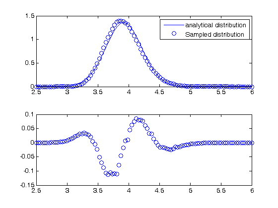
not that in the division example above, the result is nonlinear in x. You can actually see that the division product does not have a normal distribution if we look. It is subtle in this case, but when we look at the residual error between the analytical distribution and sampled distribution, you can see the errors are not random, indicating the normal distribution is not the correct model for the distribution of F/x. F/x is approximately normally distributed, so the normal distribution statistics are good estimates in this case. but that may not always be the case.

bins = linspace(2.5,6);
counts = hist(d,bins);

mu = mean(d);
sigma = std(d);

see Post 1005 .

bin_width = (max(bins)-min(bins))/length(bins);
subplot(2,1,1)
plot(bins,1/sqrt(2*pi*sigma^2)*exp(-((bins-mu).^2)./(2*sigma^2)),...
    bins,counts/N/bin_width,'bo')
legend('analytical distribution','Sampled distribution')
subplot(2,1,2)
% residual error between sampled and analytical distribution
diffs = (1/sqrt(2*pi*sigma^2)*exp(-((bins-mu).^2)./(2*sigma^2)))...
    -counts/N/bin_width;
plot(bins,diffs,'bo')
% You can see the normal distribution systematically over and under
% estimates the sampled distribution in places.

analytical stddev for division

std_d = sqrt((F_sigma/F_mu)^2 + (x_sigma/x_mu)^2)*F_mu/x_mu
std_d =

    0.2899

exponents

this rule is different than multiplication (A^2 = A*A) because in the previous examples we assumed the errors in A and B for A*B were uncorrelated. in A*A, the errors are not uncorrelated, so there is a different rule for error propogation.

t_mu = 2.03; t_sigma = 0.01*t_mu; % 1% error
A_mu = 16.07; A_sigma = 0.06;

t = t_mu + t_sigma*randn(N,1);
A = A_mu + A_sigma*randn(N,1);

Compute t^5 and sqrt(A) with error propogation

Numerical relative error

std(t.^5)
ans =

    1.7252

Analytical error

(5*t_sigma/t_mu)*t_mu^5
ans =

    1.7237

Compute sqrt(A) with error propogation

std(sqrt(A))
ans =

    0.0075

1/2*A_sigma/A_mu*sqrt(A_mu)
ans =

    0.0075

the chain rule in error propogation

let v = v0 + a*t, with uncertainties in vo,a and t

vo_mu = 1.2; vo_sigma = 0.02;
a_mu = 3; a_sigma = 0.3;
t_mu = 12; t_sigma = 0.12;

vo = vo_mu + vo_sigma*randn(N,1);
a = a_mu + a_sigma*randn(N,1);
t = t_mu + t_sigma*randn(N,1);

v = vo + a.*t;
std(v)
ans =

    3.6167

here is the analytical std dev.

sqrt(vo_sigma^2 + t_mu^2*a_sigma^2 + a_mu^2*t_sigma^2)
ans =

    3.6180

Summary

You can numerically perform error propogation analysis if you know the underlying distribution of errors on the parameters in your equations. One benefit of the numerical propogation is you don't have to remember the error propogation rules. Some limitations of this approach include

  1. You have to know the distribution of the errors in the parameters
  2. You have to assume the errors in parameters are uncorrelated.
% categories: statistics
Read and Post Comments

Random thoughts

| categories: statistics | View Comments

random_thoughts

Contents

Random thoughts

John Kitchin

clear all; close all; clc

Random numbers in Matlab

Random numbers are used in a variety of simulation methods, most notably Monte Carlo simulations. In another later post, we will see how we can use random numbers for error propogation analysis. First, we discuss two types of pseudorandom numbers we can use in Matlab: uniformly distributed and normally distributed numbers.

Uniformly distributed pseudorandom numbers

the :command:`rand` generates pseudorandom numbers uniformly distributed between 0 and 1, but not including either 0 or 1.

Single random numbers

Say you are the gambling type, and bet your friend $5 the next random number will be greater than 0.49

n = rand
if n > 0.49
    'You win!'
else
    'You lose ;('
end
n =

    0.6563


ans =

You win!

Arrays of random numbers

The odds of you winning the last bet are slightly stacked in your favor. There is only a 49% chance your friend wins, but a 51% chance that you win. Lets play the game 100,000 times and see how many times you win, and your friend wins. First, lets generate 100,000 numbers and look at the distribution with a histogram.

N = 100000;
games = rand(N,1);
nbins = 20;
hist(games,nbins)
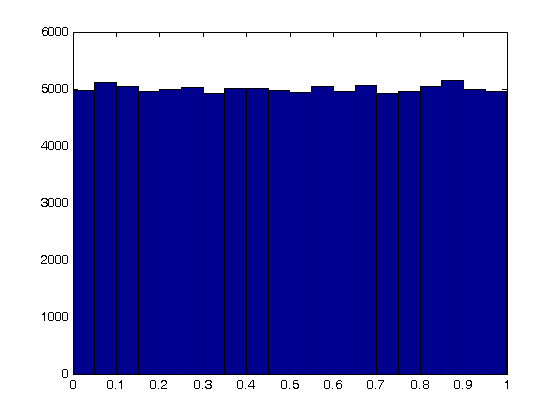
% Note that each bin has about 5000 elements. Some have a few more, some a
% few less.

Now, lets count the number of times you won.

wins = sum(games > 0.49)
losses = sum(games <= 0.49)

sprintf('percent of games won is %1.2f',(wins/N*100))
% the result is close to 51%. If you run this with 1,000,000 games, it gets
% even closer.
wins =

       51038


losses =

       48962


ans =

percent of games won is 51.04

random integers uniformly distributed over a range

the rand command gives float numbers between 0 and 1. If you want a random integer, use the randi command.

randi([1 100]) % get a random integer between 1 and 100
randi([1 100],3,1) % column vector of three integers
randi([1 100],1,3) % row vector of three integers
ans =

    65


ans =

    30
    89
    85


ans =

    62     5    97

Normally distributed numbers

The normal distribution is defined by $f(x)=\frac{1}{\sqrt{2\pi \sigma^2}} \exp (-\frac{(x-\mu)^2}{2\sigma^2})$ where $\mu$ is the mean value, and $\sigma$ is the standard deviation. In the standard distribution, $\mu=0$ and $\sigma=1$.

mu = 0; sigma=1;

get a single number

R = mu + sigma*randn
R =

   -0.4563

get a lot of normally distributed numbers

N = 100000;
samples = mu + sigma*randn(N,1);

We define our own bins to do the histogram on

bins = linspace(-5,5);
% and get the counts in each bin also
counts = hist(samples, bins);

Comparing the random distribution to the normal distribution

to compare our sampled distribution to the analytical normal distribution, we have to normalize the histogram. The probability density of any bin is defined by the number of counts for that bin divided by the total number of samples divided by the width

the bin width is the range of bins divided by the number of bins.

bin_width = (max(bins)-min(bins))/length(bins);
plot(bins,1/sqrt(2*pi*sigma^2)*exp(-((bins-mu).^2)./(2*sigma^2)),...
    bins,counts/N/bin_width,'bo')
legend('analytical distribution','Sampled distribution')
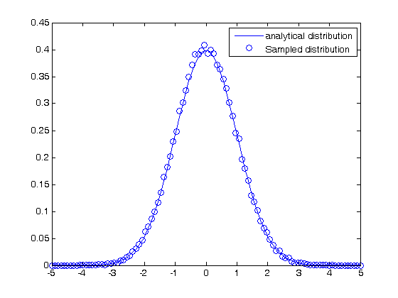
% For the most part, you can see the two distributions agree. There is some
% variation due to the sampled distribution having a finite number of
% samples. As you increase the sample size, the agreement gets better and
% better.

some properties of the normal distribution

What fraction of points lie between plus and minus one standard deviation of the mean?

samples >= mu-sigma will return a vector of ones where the inequality is true, and zeros where it is not. (samples >= mu-sigma) & (samples <= mu+sigma) will return a vector of ones where there is a one in both vectors, and a zero where there is not. In other words, a vector where both inequalities are true. Finally, we can sum the vector to get the number of elements where the two inequalities are true, and finally normalize by the total number of samples to get the fraction of samples that are greater than -sigma and less than sigma.

a1 = sum((samples >= mu-sigma) & (samples <= mu+sigma))/N*100;
sprintf('%1.2f %% of the samples are within plus or minus one standard deviation of the mean.',a1)
ans =

68.44 % of the samples are within plus or minus one standard deviation of the mean.

What fraction of points lie between plus and minus two standard deviations of the mean?

a2 = sum((samples >= mu - 2*sigma) & (samples <= mu + 2*sigma))/N*100;
sprintf('%1.2f %% of the samples are within plus or minus two standard deviations of the mean.',a2)
% this is where the rule of thumb that a 95% confidence interval is plus or
% minus two standard deviations from the mean.
ans =

95.48 % of the samples are within plus or minus two standard deviations of the mean.

Summary

Matlab has a variety of tools for generating pseudorandom numbers of different types. Keep in mind the numbers are only pseudorandom, but they are still useful for many things as we will see in future posts.
% categories: statistics
% tags: math
Read and Post Comments

Know your tolerance

| categories: nonlinear algebra | View Comments

Know your tolerance

Know your tolerance

Given:

Contents

$$V = \frac{\nu (C_{Ao} - C_A)}{k C_A^2}$$

with the information given below, solve for the exit concentration. This should be simple. We use the units package to make sure we don't miss any units.

clear all; close all; clc
u = cmu.units;

Cao = 2*u.mol/u.L;
V = 10*u.L;
nu = 0.5*u.L/u.s;
k = 0.23 * u.L/u.mol/u.s;

function we need to solve

f = @(Ca) V - nu*(Cao - Ca)./(k*Ca.^2);

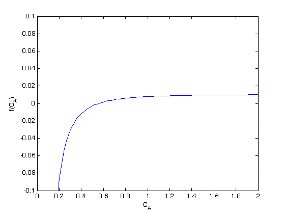
plot the function to estimate the solution

c = linspace(0,2)*u.mol/u.L;
plot(c/(u.mol/u.L),f(c))
ylim([-0.1 0.1]) % limit the y-range to see the zero easier
xlabel('C_A')
ylabel('f(C_A)')
% we want the value of C_A that makes f(C_A)=0. this happens around C_A=0.5
cguess = 0.5*u.mol/u.L;
c = fsolve(f,cguess)
% it is a little weird that the solution is the same as our initial guess.
% Usually the answer is at least a little different!
Equation solved at initial point.

fsolve completed because the vector of function values at the initial point
is near zero as measured by the default value of the function tolerance, and
the problem appears regular as measured by the gradient.


ans =

  500.0000


Equation solved at initial point.

fsolve completed because the vector of function values at the initial point
is near zero as measured by the default value of the function tolerance, and
the problem appears regular as measured by the gradient.


500/m^3*mol

check your solution

z = f(c)
z.as(u.L)
% this is not really that close to zero, especially when you look at the
% units in L!
-0.00304348*m^3

ans =

-3.043*L

closer look at fsolve

Let's output some more information.

options = optimset('Display','iter');
[X,FVAL,EXITFLAG,OUTPUT] = fsolve(f,cguess,options)
% It should be a warning that zero iterations were taken! Our guess was
% probably not that good! The EXITFLAG=1 means the function ended ok as far
% as fsolve is concerned.
                                         Norm of      First-order   Trust-region
 Iteration  Func-count     f(x)          step         optimality    radius
     0          2    9.26276e-006                     1.85e-007               1

Equation solved at initial point.

fsolve completed because the vector of function values at the initial point
is near zero as measured by the default value of the function tolerance, and
the problem appears regular as measured by the gradient.


ans =

  500.0000


                                         Norm of      First-order   Trust-region
 Iteration  Func-count     f(x)          step         optimality    radius
     0          2    9.26276e-006                     1.85e-007               1

Equation solved at initial point.

fsolve completed because the vector of function values at the initial point
is near zero as measured by the default value of the function tolerance, and
the problem appears regular as measured by the gradient.


500/m^3*mol
-0.00304348*m^3

EXITFLAG =

     1


OUTPUT = 

       iterations: 0
        funcCount: 2
        algorithm: 'trust-region dogleg'
    firstorderopt: 1.8526e-007
          message: [1x756 char]

The problem is bad scaling because the underlying units are stored in m^3, which results in very small numbers that are close to zero. So, fsolve sees a number it thinks is close to zero, and stops. One way to fix this is to decrease the tolerance on what constitutes zero.

options = optimset('TolFun',1e-9);
cguess = 0.5*u.mol/u.L;
[c2,FVAL,EXITFLAG,OUTPUT] = fsolve(f,cguess,options)
z2 = f(c2)
z2.as(u.L) % much closer to zero.

sprintf('The exit concentration is %1.2f mol/L', c2/(u.mol/u.L))
Equation solved.

fsolve completed because the vector of function values is near zero
as measured by the selected value of the function tolerance, and
the problem appears regular as measured by the gradient.


ans =

  559.5545


Equation solved.

fsolve completed because the vector of function values is near zero
as measured by the selected value of the function tolerance, and
the problem appears regular as measured by the gradient.


559.554/m^3*mol
-1.24874e-006*m^3

EXITFLAG =

     1


OUTPUT = 

       iterations: 6
        funcCount: 14
        algorithm: 'trust-region dogleg'
    firstorderopt: 5.3309e-011
          message: [1x698 char]

-1.24874e-006*m^3

ans =

-0.001*L


ans =

The exit concentration is 0.56 mol/L

Rescaling the units

We can make the default length unit be dm, then the default volume unit will be 1L (dm^3). This will effectively rescale the function so that the default tolerance will be effective. Note you have to specify the unit for each unit in the order (length, time, mass, temperature, charge, mol).

u = cmu.unit.units('dm','s','kg','K','coul','mol');
Cao = 2*u.mol/u.L;
V = 10*u.L;
nu = 0.5*u.L/u.s;
k = 0.23 * u.L/u.mol/u.s;

% function we need to solve
f = @(Ca) V - nu*(Cao - Ca)./(k*Ca.^2);
cguess = 0.5*u.mol/u.L;
[c3,FVAL,EXITFLAG,OUTPUT] = fsolve(f,cguess)
sprintf('The exit concentration is %1.2f', c3)
% we were able to solve this more reasonably scaled problem without
% changing any default tolerances.
Equation solved.

fsolve completed because the vector of function values is near zero
as measured by the default value of the function tolerance, and
the problem appears regular as measured by the gradient.


ans =

    0.5596


Equation solved.

fsolve completed because the vector of function values is near zero
as measured by the default value of the function tolerance, and
the problem appears regular as measured by the gradient.


0.559584/dm^3*mol
-3.9293e-012*dm^3

EXITFLAG =

     1


OUTPUT = 

       iterations: 4
        funcCount: 10
        algorithm: 'trust-region dogleg'
    firstorderopt: 1.6772e-010
          message: [1x695 char]


ans =

The exit concentration is 0.56 (dm^3*mol)^-1

'done'
% categories: nonlinear algebra
% tags: reaction engineering, units
ans =

done

Read and Post Comments

Stopping the integration of an ODE at some condition

| categories: odes | View Comments

Stopping the integration of an ODE at some condition

Stopping the integration of an ODE at some condition

John Kitchin

In Post 968 we learned how to get the numerical solution to an ODE, and then to use the deval function to solve the solution for a particular value. The deval function uses interpolation to evaluate the solution at other valuse. An alternative approach would be to stop the ODE integration when the solution has the value you want. That can be done in Matlab by using an "event". You setup an event function and tell the ode solver to use it by setting an option.

Contents

The problem

given that the concentration of a species A in a constant volume, batch reactor obeys this differential equation $\frac{dC_A}{dt}=- k C_A^2$ with the initial condition $C_A(t=0) = 2.3$ mol/L and $k = 0.23$ L/mol/s, compute the time it takes for $C_A$ to be reduced to 1 mol/L.

function main
clear all; close all; clc

k = 0.23;
Cao = 2.3;
tspan = [0 10];

% create an options variable
options = odeset('Events',@event_function);

% note the extra outputs
[t,Ca,TE,VE] = ode45(@myode,tspan,Cao,options);
TE % this is the time value where the event occurred
VE % this is the value of Ca where the event occurred

sprintf('At t = %1.2f seconds the concentration of A is %1.2f mol/L.', TE,VE)
TE =

    2.4598


VE =

    1.0000


ans =

At t = 2.46 seconds the concentration of A is 1.00 mol/L.

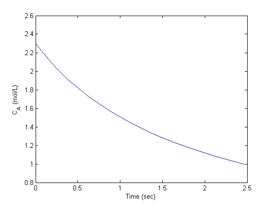
plot(t,Ca)
xlabel('Time (sec)')
ylabel('C_A (mol/L)')
% you can see the integration terminated at Ca = 1
'done'
ans =

done

function dCadt = myode(t,Ca)
k = 0.23;
dCadt = -k*Ca^2;

function [value,isterminal,direction] = event_function(t,Ca)
% when value is equal to zero, an event is triggered.
% set isterminal to 1 to stop the solver at the first event, or 0 to
% get all the events.
%  direction=0 if all zeros are to be computed (the default), +1 if
%  only zeros where the event function is increasing, and -1 if only
%  zeros where the event function is decreasing.
value = Ca - 1.0;  % when value = 0, an event is triggered
isterminal = 1; % terminate after the first event
direction = 0;  % get all the zeros
% categories: ODEs
% tags: reaction engineering
Read and Post Comments

« Previous Page -- Next Page »