Numerical propogation of errors

Propogation of errors is essential to understanding how the uncertainty in a parameter affects computations that use that parameter. The uncertainty propogates by a set of rules into your solution. These rules are not easy to remember, or apply to complicated situations, and are only approximate for equations that are nonlinear in the parameters.

We will use a Monte Carlo simulation to illustrate error propogation. The idea is to generate a distribution of possible parameter values, and to evaluate your equation for each parameter value. Then, we perform statistical analysis on the results to determine the standard error of the results.

We will assume all parameters are defined by a normal distribution with known mean and standard deviation.

Contents

adapted from here.

clear all;

N= 1e6; % # of samples of parameters

Error propogation for addition and subtraction

A_mu = 2.5; A_sigma = 0.4;
B_mu = 4.1; B_sigma = 0.3;

A = A_mu + A_sigma*randn(N,1);
B = B_mu + B_sigma*randn(N,1);

p = A + B;
m = A - B;

std(p)
std(m)

ans =

    0.4999


ans =

    0.4997

here is the analytical std dev of these two quantities. It agrees with the numerical answers above

sqrt(A_sigma^2 + B_sigma^2)

ans =

    0.5000

multiplication and division

F_mu = 25; F_sigma = 1;
x_mu = 6.4; x_sigma = 0.4;

F = F_mu + F_sigma*randn(N,1);
x = x_mu + x_sigma*randn(N,1);

Multiplication

t = F.*x;
std(t)

ans =

   11.8721

analytical stddev for multiplication

std_t = sqrt((F_sigma/F_mu)^2 + (x_sigma/x_mu)^2)*F_mu*x_mu

std_t =

   11.8727

division

this is really like multiplication: F/x = F * 1/x

d = F./x;
std(d)

ans =

    0.2938

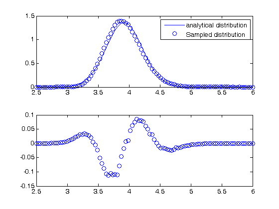
not that in the division example above, the result is nonlinear in x. You can actually see that the division product does not have a normal distribution if we look. It is subtle in this case, but when we look at the residual error between the analytical distribution and sampled distribution, you can see the errors are not random, indicating the normal distribution is not the correct model for the distribution of F/x. F/x is approximately normally distributed, so the normal distribution statistics are good estimates in this case. but that may not always be the case.

bins = linspace(2.5,6);
counts = hist(d,bins);

mu = mean(d);
sigma = std(d);

see Post 1005 .

bin_width = (max(bins)-min(bins))/length(bins);
subplot(2,1,1)
plot(bins,1/sqrt(2*pi*sigma^2)*exp(-((bins-mu).^2)./(2*sigma^2)),...
    bins,counts/N/bin_width,'bo')
legend('analytical distribution','Sampled distribution')
subplot(2,1,2)
% residual error between sampled and analytical distribution
diffs = (1/sqrt(2*pi*sigma^2)*exp(-((bins-mu).^2)./(2*sigma^2)))...
    -counts/N/bin_width;
plot(bins,diffs,'bo')
% You can see the normal distribution systematically over and under
% estimates the sampled distribution in places.

analytical stddev for division

std_d = sqrt((F_sigma/F_mu)^2 + (x_sigma/x_mu)^2)*F_mu/x_mu

std_d =

    0.2899

exponents

this rule is different than multiplication (A^2 = A*A) because in the previous examples we assumed the errors in A and B for A*B were uncorrelated. in A*A, the errors are not uncorrelated, so there is a different rule for error propogation.

t_mu = 2.03; t_sigma = 0.01*t_mu; % 1% error
A_mu = 16.07; A_sigma = 0.06;

t = t_mu + t_sigma*randn(N,1);
A = A_mu + A_sigma*randn(N,1);

Compute t^5 and sqrt(A) with error propogation

Numerical relative error

std(t.^5)

ans =

    1.7252

Analytical error

(5*t_sigma/t_mu)*t_mu^5

ans =

    1.7237

Compute sqrt(A) with error propogation

std(sqrt(A))

ans =

    0.0075

1/2*A_sigma/A_mu*sqrt(A_mu)

ans =

    0.0075

the chain rule in error propogation

let v = v0 + a*t, with uncertainties in vo,a and t

vo_mu = 1.2; vo_sigma = 0.02;
a_mu = 3; a_sigma = 0.3;
t_mu = 12; t_sigma = 0.12;

vo = vo_mu + vo_sigma*randn(N,1);
a = a_mu + a_sigma*randn(N,1);
t = t_mu + t_sigma*randn(N,1);

v = vo + a.*t;

std(v)

ans =

    3.6167

here is the analytical std dev.

sqrt(vo_sigma^2 + t_mu^2*a_sigma^2 + a_mu^2*t_sigma^2)

ans =

    3.6180

Summary

You can numerically perform error propogation analysis if you know the underlying distribution of errors on the parameters in your equations. One benefit of the numerical propogation is you don't have to remember the error propogation rules. Some limitations of this approach include

% categories: statistics

Published with MATLAB® 7.10