Vectorized piecewise functions

| categories: miscellaneous | View Comments

vectorized_piecewise

Contents

Vectorized piecewise functions

John Kitchin

Occasionally we need to define piecewise functions, e.g.

$$f(x) = \begin{array}{l}
0, x<0 \\
x, 0 <= x < 1\\
2-x, 1 < x <= 2\\
0, x> 2
\end{array}$$

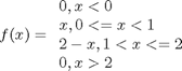
Today we examine a few ways to define a function like this.

function main
clear all; clc; close all

Use conditional statements in a function

    function y = f1(x)
        if x < 0
            y = 0;
        elseif x >= 0 & x < 1
            y = x;
        elseif x >= 1 & x < 2
            y = 2-x;
        else
            y = 0;
        end
    end

This works, but the function is not vectorized, i.e. f([-1 0 2 3]) does not evaluate at all, you get an error. You can get vectorized behavior by using the arrayfun function, or by writing your own loop. This doesn't fix all limitations, for example you cannot use the f1 function in the quad function to integrate it.

x = linspace(-1,3);
plot(x,arrayfun(@f1,x))
y = zeros(size(x));
for i=1:length(y)
    y(i) = f1(x(i));
end
plot(x,y)

Neither of those methods is convenient. It would be nicer if the function was vectorized, which would allow the direct notation f1([0 1 2 3 4]). A simple way to achieve this is through the use of logical arrays. We create logical arrays from comparison statements

x = linspace(-1,3,10)
x < 0
x =

  Columns 1 through 6

   -1.0000   -0.5556   -0.1111    0.3333    0.7778    1.2222

  Columns 7 through 10

    1.6667    2.1111    2.5556    3.0000


ans =

     1     1     1     0     0     0     0     0     0     0

x >= 0 & x < 1
ans =

     0     0     0     1     1     0     0     0     0     0

We can use the logical arrays as masks on functions; where the logical array is 1, the function value will be used, and where it is zero, the function value will not be used.

    function y = f2(x)
        % vectorized piecewise function
        % we start with zeros for all values of y(x)
        y = zeros(size(x));
        % now we add the functions, masked by the logical arrays.
        y = y + (x >= 0 & x < 1).*x;
        y = y + (x >= 1 & x < 2).*(2-x);
    end


x = linspace(-1,3);
plot(x,f2(x))

And now we can integrate it with quad!

quad(@f2,-1,3)
ans =

    1.0000

Third approach with Heaviside functions

The Heaviside function is defined to be zero for x less than some value, and 0.5 for x=0, and 1 for x >= 0. If you can live with y=0.5 for x=0, you can define a vectorized function in terms of Heaviside functions like this.

    function y = f3(x)
        y1 = (heaviside(x) - heaviside(x-1)).*x ; % first interval
        y2 = (heaviside(x-1) - heaviside(x-2)).*(2-x); % 2nd interval
        y = y1 + y2; % both intervals
    end

plot(x,f3(x))
quad(@f3,-1,3)
ans =

    1.0000

Summary

There are many ways to define piecewise functions, and vectorization is not always necessary. The advantages of vectorization are usually notational simplicity and speed; loops in Matlab are usually very slow compared to vectorized functions.

end

% categories: Miscellaneous
% tags: vectorization
Read and Post Comments

Matlab meets the steam tables

| categories: miscellaneous | View Comments

Matlab meets the steam tables

Matlab meets the steam tables

John Kitchin

A Matlab module for the steam tables is available for download at http://www.x-eng.com/XSteam_Matlab.htm. To do this example yourself, you need to download this zipfile and unzip it into your Matlab path. Today we will examine using this module for examining the Rankine power generation cycle, following example3.7-1 in Sandler's Thermodynamics book.

Problem statement: A Rankine cycle operates using steam with the condenser at 100 degC, a pressure of 3.0 MPa and temperature of 600 degC in the boiler. Assuming the compressor and turbine operate reversibly, estimate the efficiency of the cycle.

We will use the XSteam module to compute the required properties. There is only one function in XSteam, which takes a string and one or two arguments. The string specifies which subfunction to use.

We will use these functions from the module.

Contents

psat_T Saturation pressure (bar) at a specific T in degC
sL_T   Entropy (kJ/kg/K) of saturated liquid at T(degC)
hL_T   Enthalpy (kJ/kg)of saturated liquid at T(degC)
vL_T   Saturated liquid volume (m^3/kg)
T_ps   steam Temperature (degC) for a given pressure (bar) and entropy (kJ/kg/K)
h_pt   steam enthalpy (kJ/kg) at a given pressure (bar) and temperature (degC)
s_pt   steam entropy (kJ/kg/K) at a given pressure (bar) and temperature (degC)

We will use the cmu.units package to keep track of the units. Remember that the units package internally stores units in terms of base units, so to get a pressure in bar, we use the syntax P/u.bar, which is a dimensionless number with a magnitude equal to the number of bar.

clear all; clc; close all
u = cmu.units;

Starting point in the Rankine cycle in condenser.

we have saturated liquid here, and we get the thermodynamic properties for the given temperature.

T1 = 100; % degC
P1 = XSteam('psat_T',T1)*u.bar;
s1 = XSteam('sL_T', T1)*u.kJ/u.kg/u.K;
h1 = XSteam('hL_t', T1)*u.kJ/u.kg;
v1 = XSteam('vL_T', T1)*u.m^3/u.kg; % we need this to compute compressor work

isentropic compression of liquid to point 2

The final pressure is given, and we need to compute the new temperatures, and enthalpy.

P2 = 3*u.MPa;
s2 = s1;  % this is what isentropic means
T2 = XSteam('T_ps',P2/u.bar, s1/(u.kJ/u.kg/u.K));
h2 = XSteam('h_pt', P2/u.bar,T2)*u.kJ/u.kg;

% work done to compress liquid. This is an approximation, since the
% volume does change a little with pressure, but the overall work here
% is pretty small so we neglect the volume change.
WdotP = v1*(P2-P1);
fprintf('the compressor work is: %s\n', WdotP.as(u.kJ/u.kg,'%1.2f'))
the compressor work is: 3.02*kJ/kg

isobaric heating to T3 in Boiler where we make steam

T3 = 600; % degC
P3 = P2; % this is what isobaric means
h3 = XSteam('h_pt', P3/u.bar, T3)*u.kJ/u.kg;
s3 = XSteam('s_pt', P3/u.bar, T3)*u.kJ/u.kg/u.K;

Qb = h3 - h2; % heat required to make the steam
fprintf('the boiler heat duty is: %s\n', Qb.as(u.kJ/u.kg,'%1.2f'))
the boiler heat duty is: 3260.68*kJ/kg

isentropic expansion through turbine to point 4

Still steam

T4 = XSteam('T_ps',P1/u.bar, s3/(u.kJ/u.kg/u.K));
h4 = XSteam('h_pt', P1/u.bar, T4)*u.kJ/u.kg;
s4 = s3; % isentropic
Qc = h4 - h1; % work required to cool from T4 to T1 in the condenser
fprintf('the condenser heat duty is: %s\n', Qc.as(u.kJ/u.kg,'%1.2f'))
the condenser heat duty is: 2316.99*kJ/kg

This heat flow is not counted against the overall efficiency. Presumably a heat exchanger can do this cooling against the cooler environment, so only heat exchange fluid pumping costs would be incurred.

to get from point 4 to point 1

WdotTurbine = h4 - h3; % work extracted from the expansion
fprintf('the turbine work is: %s\n', WdotTurbine.as(u.kJ/u.kg,'%1.2f'))
the turbine work is: -946.72*kJ/kg

efficiency

This is a ratio of the work put in to make the steam, and the net work obtained from the turbine. The answer here agrees with the efficiency calculated in Sandler on page 135.

eta = -(WdotTurbine - WdotP)/Qb

fprintf('the overall efficiency is %1.0f%%\n', (eta*100))
eta =

   0.291271696419079

the overall efficiency is 29%

Entropy-temperature chart

The XSteam module makes it pretty easy to generate figures of the steam tables. Here we generate an entropy-Temperature graph.

T = linspace(0,800,200); % range of temperatures

figure; hold on
% we need to compute S-T for a range of pressures. Here
for P = [0.01 0.1 1 5 30 100 250 500 1000] % bar
    % XSteam is not vectorized, so here is an easy way to compute a
    % vector of entropies
    S = arrayfun(@(t) XSteam('s_PT',P,t),T);
    plot(S,T,'k-')
    text(S(end),T(end),sprintf('%1.1f bar',P),'rotation',90)
end
set(gca,'Position',[0.13 0.11 0.775 0.7])

% saturated vapor and liquid entropy lines
svap = arrayfun(@(t) XSteam('sV_T',t),T);
sliq = arrayfun(@(t) XSteam('sL_T',t),T);

plot(svap,T,'r-')
plot(sliq,T,'b-')
xlabel('Entropy (kJ/(kg K)')
ylabel('Temperature (^\circC)')

Plot Path

The path from 1 to 2 is isentropic, and has a small T change.

plot([s1 s2]/(u.kJ/u.kg/u.K),...
    [T1 T2],'ro ','markersize',8,'markerfacecolor','r')

% the path from 2 to 3 is isobaric
T23 = linspace(T2, T3);
S23 = arrayfun(@(t) XSteam('s_PT',P2/u.bar,t),T23);
plot(S23,T23,'b-','linewidth',4)

% the path from 3 to 4 is isentropic
plot([s3 s4]/(u.kJ/u.kg/u.K),...
    [T3 T4],'g-','linewidth',4)

% and from 4 to 1 is isobaric
T41 = linspace(T4,T1-0.01); % subtract 0.01 to get the liquid entropy
S41 = arrayfun(@(t) XSteam('s_PT',P1/u.bar,t),T41);
plot(S41,T41,'r-','linewidth',4)

Note steps 1 and 2 are very close together on this graph and hard to see.

Summary

This was an interesting exercise. On one hand, the tedium of interpolating the steam tables is gone. On the other hand, you still have to know exactly what to ask for to get an answer that is correct. The XSteam interface is a little clunky, and takes some getting used to. It would be nice if it was vectorized to avoid the arrayfun calls.

% categories: Miscellaneous
% tags: Thermodynamics
Read and Post Comments

Smooth transitions between discontinuous functions

| categories: miscellaneous, nonlinear algebra | View Comments

transition_discontinuous_functions

Contents

Smooth transitions between discontinuous functions

John Kitchin

In Post 1280 we used a correlation for the Fanning friction factor for turbulent flow in a pipe. For laminar flow (Re < 3000), there is another correlation that is commonly used: $f_F = 16/Re$. Unfortunately, the correlations for laminar flow and turbulent flow have different values at the transition that should occur at Re = 3000. This discontinuity can cause a lot of problems for numerical solvers that rely on derivatives.

Today we examine a strategy for smoothly joining these two functions.

function main
clear all; close all; clc

Friction factor correlations

    function f = fF_laminar(Re)
        f = 16./Re;
    end

    function f = fF_turbulent(Re)
        % Nikuradse correlation for turbulent flow
        function f = internalfunc(Re)
            f = fzero(@(f) 1/sqrt(f) - (4.0*log10(Re*sqrt(f))-0.4), 0.01);
        end
        % this makes the function act as if it were vectorized, so we can
        % get an array of friction factors
        f = arrayfun(@internalfunc,Re);
    end

Plot the correlations

Re1 = linspace(500,3000);
f1 = fF_laminar(Re1);

Re2 = linspace(3000,10000);
f2 = fF_turbulent(Re2);

figure(1)
plot(Re1,f1,Re2,f2)
xlabel('Re')
ylabel('f_F')

You can see the discontinuity at Re = 3000. What we need is a method to join these two functions smoothly. We can do that with a sigmoid function.

Sigmoid functions

A sigmoid function smoothly varies from 0 to 1 according to the equation: $\sigma(x) = \frac{1}{1 + e^{-(x-x0)/\alpha}}$
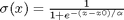
. The transition is centered on $x0$, and $\alpha$ determines the width of the transition.

x = linspace(-4,4);
y = 1./(1+exp(-x/0.1));
figure(2)
plot(x,y)
xlabel('x'); ylabel('y'); title('\sigma(x)')

If we have two functions, $f_1(x)$ and $f_2(x)$ we want to smoothly join, we do it like this: $f(x) = (1-\sigma(x))f_1(x) + \sigma(x)f_2(x)$. There is no formal justification for this form of joining, it is simply a mathematical convenience to get a numerically smooth function. Other functions besides the sigmoid function could also be used, as long as they smoothly transition from 0 to 1, or from 1 to zero.

Smoothly transitioning function to estimate friction factor

    function f = fanning_friction_factor(Re)
        % combined, continuous correlation for the fanning friction factor.
        % the alpha parameter is chosen to provide the desired smoothness.
        % The transition region is about +- 4*alpha. The value 450 was
        % selected to reasonably match the shape of the correlation
        % function provided by Morrison (see last section of this file)
        sigma =  1./(1+exp(-(Re - 3000)/450));
        f = (1-sigma).*fF_laminar(Re) + sigma.*fF_turbulent(Re);
    end

Re = linspace(500,10000);
f = fanning_friction_factor(Re);

figure(1); hold all
plot(Re,f)
xlabel('Re')
ylabel('f_F')
legend 'laminar' 'turbulent' 'smooth transition'
Exiting fzero: aborting search for an interval containing a sign change
    because complex function value encountered during search.
(Function value at -0.0028 is -5.2902-21.627i.)
Check function or try again with a different starting value.

You can see that away from the transition the combined function is practically equivalent to the original two functions. That is because away from the transition the sigmoid function is 0 or 1. Near Re = 3000 is a smooth transition from one curve to the other curve.

Morrison derived a single function for the friction factor correlation over all Re: $f = \frac{0.0076\left(\frac{3170}{Re}\right)^{0.165}}{1 + \left(\frac{3171}{Re}\right)^{7.0}} + \frac{16}{Re}$
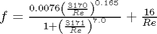
. Here we show the comparison with the approach used above. The friction factor differs slightly at high Re, becauase Morrison's is based on the Prandlt correlation, while the work here is based on the Nikuradse correlation. They are similar, but not the same.

h = plot(Re,16./Re + (0.0076*(3170./Re).^0.165)./(1 + (3170./Re).^7))

% Append an entry to the legend
[LEGH,OBJH,OUTH,OUTM] = legend;
% Add object with new handle and new legend string to legend
legend([OUTH;h],OUTM{:},'Morrison')
h =

  415.0735

Summary

The approach demonstrated here allows one to smoothly join two discontinuous functions that describe physics in different regimes, and that must transition over some range of data. It should be emphasized that the method has no physical basis, it simply allows one to create a mathematically smooth function, which could be necessary for some optimizers or solvers to work.

end % main

% categories: Miscellaneous, nonlinear algebra
% tags: Fluids
Read and Post Comments

Using Java inside Matlab

| categories: data analysis, miscellaneous | View Comments

Using Java inside Matlab

Using Java inside Matlab

John Kitchin

Matlab is pretty good, but it doesn't do everything, and you might not always have the toolbox that contains the function you want. There might even be an excellent open-source software library that can't be included in Matlab, but can be used within Matlab.

Matlab has excellent support for using Java with minimal effort. A repository of numerical libraries can be found at http://math.nist.gov/javanumerics/. In this example we install the commons-math Java library, and show an example of using it.

Contents

Here are a few things the commons libary can do:

  Computing means, variances and other summary statistics for a list of numbers
  Fitting a line to a set of data points using linear regression
  Finding a smooth curve that passes through a collection of points (interpolation)
  Fitting a parametric model to a set of measurements using least-squares methods
  Solving equations involving real-valued functions (i.e. root-finding)
  Solving systems of linear equations
  Solving Ordinary Differential Equations
  Minimizing multi-dimensional functions
  Generating random numbers with more restrictions (e.g distribution, range) than what is possible using the JDK
  Generating random samples and/or datasets that are "like" the data in an input file
  Performing statistical significance tests
  Miscellaneous mathematical functions such as factorials, binomial coefficients and "special functions" (e.g. gamma, beta functions)

Many of them duplicate features in Matlab, but they may implement different algorithms, or more convenient syntax.

clear all; clc; close all

download and install

These two commands only need to be run once, so comment them out after you run them.

%urlwrite('http://mirror.metrocast.net/apache/commons/math/binaries/commons-math-2.2.zip','commons-math-2.2.zip')
%unzip('commons-math-2.2.zip')

We have to add the jar file to the javaclasspath so we can use it.

javaaddpath([pwd '/commons-math-2.2/commons-math-2.2.jar'])

linear regression with Matlab

Note that the regress command is part of the Statistics toolbox, which is great if you have it! We show here how to do it, so we also have something to compare the Java result to.

x = [1 2 3 4 5]';
y = [3 5 7 14 11]';

[b bint]= regress(y,[x.^0 x])
b =

    0.5000
    2.5000


bint =

   -7.5615    8.5615
    0.0694    4.9306

Now the Java way

Documentation Examples

The first thing we do is import the Java library. the * at the end indicates that all classes should be imported.

import org.apache.commons.math.stat.regression.*

Create a class instance.

The SimpleRegression class has several methods that we can call later to perform analysis

regression = SimpleRegression();
methods(regression)
Methods for class org.apache.commons.math.stat.regression.SimpleRegression:

SimpleRegression            getSlope                    
addData                     getSlopeConfidenceInterval  
clear                       getSlopeStdErr              
equals                      getSumSquaredErrors         
getClass                    getTotalSumSquares          
getIntercept                hashCode                    
getInterceptStdErr          notify                      
getMeanSquareError          notifyAll                   
getN                        predict                     
getR                        toString                    
getRSquare                  wait                        
getRegressionSumSquares     
getSignificance             

add the data

regression.addData([x y]);

get the slope and some statistics of the slope

m = regression.getSlope()
mstd = regression.getSlopeStdErr()
mint = regression.getSlopeConfidenceInterval(); % 95% by default
[m - mint  m + mint] % this is the 95% interval
m =

    2.5000


mstd =

    0.7638


ans =

    0.0694    4.9306

Note the confidence interval is greater than +- 2*sigma. This is because of the student-t table multiplier on the standard error due to the small number

get the intercept and some statistics

note there is not getInterceptConfidenceInterval method for some reason!

b = regression.getIntercept()
bstd = regression.getInterceptStdErr()

sprintf('R^2 = %1.3f', regression.getRSquare())
b =

    0.5000


bstd =

    2.5331


ans =

R^2 = 0.781

Summary

It takes more lines of code to get the Java version of linear regression, but you have finer control over what data you get, and what order you get it in. You still have to read the Java documentation to learn the command syntax, and debugging can be somewhat more difficult than straight Matlab. However, the integration of Java into Matlab opens some interesting possibilities to extend Matlab's functionality.

% categories: Miscellaneous, data analysis
Read and Post Comments

Create a word document from Matlab

| categories: miscellaneous | View Comments

Create a word document from Matlab

Create a word document from Matlab

John Kitchin

Have you been wondering how to create a word document from Matlab that doesn't require the publish button? Below we look at a way to use Matlab for COM automation to create a word document and put text in it. I adapted the Perl code at http://www.adp-gmbh.ch/perl/word.html for this example. There is hardly any interesting output from any of these commands,

Contents

Create the word application

and make it visible

word = actxserver('Word.Application');
word.Visible = 1;

Add a new document and get the current selection

document = word.Documents.Add;
selection = word.Selection;

add text and paragraphs

selection.TypeText('Hello world. ');
selection.TypeText('My name is Professor Kitchin');
selection.TypeParagraph;
selection.TypeText('How are you today?');
selection.TypeParagraph;

Setting a Header

selection.TypeText('Big Finale');
selection.Style='Heading 1';
selection.TypeParagraph;

Modifying Header properties

H1 = document.Styles.Item('Heading 1')
H1.Font.Name = 'Garamond';
H1.Font.Size = 20;
H1.Font.Bold = 1;
H1.Font.TextColor.RGB=60000; % some ugly color green

selection.TypeParagraph
selection.TypeText('That is all for today!')
 
H1 =
 
	Interface.0002092C_0000_0000_C000_000000000046

Now we save the document

document.SaveAs2([pwd '/test.docx']);
word.Quit();

Summary

That is it! I wouldn't call this extra convenient, but if you have a need to automate the production of Word documents from a program, this is an approach that you can use. You may find http://msdn.microsoft.com/en-us/library/kw65a0we%28v=vs.80%29.aspx a helpful link for documentation of what you can do.

%  download test.docx 

% categories: Miscellaneous
Read and Post Comments

« Previous Page