Gibbs energy minimization and the NIST webbook
December 26, 2011 at 01:10 AM | categories: optimization | View Comments
Gibbs energy minimization and the NIST webbook
John Kitchin
Contents
- Links to data
- We define species like this.
- Heats of formation at 298.15 K
- Shomate parameters for each species
- Shomate equations
- Gibbs energy of mixture
- Elemental conservation constraints
- Constraints on bounds
- Solve the minimization problem
- Compute mole fractions and partial pressures
- Computing equilibrium constants
In Post 1536 we used the NIST webbook to compute a temperature dependent Gibbs energy of reaction, and then used a reaction extent variable to compute the equilibrium concentrations of each species for the water gas shift reaction.
Today, we look at the direct minimization of the Gibbs free energy of the species, with no assumptions about stoichiometry of reactions. We only apply the constraint of conservation of atoms. We use the NIST Webbook to provide the data for the Gibbs energy of each species.
As a reminder we consider equilibrium between the species  ,
,  ,
,  and
and  , at 1000K, and 10 atm total pressure with an initial equimolar molar flow rate of and .
Links to data
function nist_wb_constrained_min
T = 1000; %K
R = 8.314e-3; % kJ/mol/K

P = 10; % atm, this is the total pressure in the reactor
Po = 1; % atm, this is the standard state pressure
We define species like this.
We are going to store all the data and calculations in vectors, so we need to assign each position in the vector to a species. Here are the definitions we use in this work.
1  CO
2  H2O
3  CO2
4  H2
species = {'CO' 'H2O' 'CO2' 'H2'};
Heats of formation at 298.15 K
Hf298 = [
    -110.53  % CO
    -241.826 % H2O
    -393.51  % CO2
       0.0]; % H2
Shomate parameters for each species
A B C D E F G H
WB = [25.56759  6.096130     4.054656  -2.671301  0.131021 -118.0089 227.3665   -110.5271  % CO
      30.09200  6.832514     6.793435  -2.534480  0.082139 -250.8810 223.3967   -241.8264    % H2O
      24.99735  55.18696   -33.69137    7.948387 -0.136638 -403.6075 228.2431   -393.5224   % CO2
      33.066178 -11.363417  11.432816  -2.772874 -0.158558 -9.980797 172.707974    0.0]; % H2
Shomate equations
t = T/1000;
T_H = [t; t^2/2; t^3/3; t^4/4; -1/t; 1; 0; -1];
T_S = [log(t); t; t^2/2; t^3/3; -1/(2*t^2); 0; 1; 0];

H = WB*T_H; % (H - H_298.15) kJ/mol
S = WB*T_S/1000; % absolute entropy kJ/mol/K

Gjo = Hf298 + H - T*S; % Gibbs energy of each component at 1000 K
Gibbs energy of mixture
this function assumes the ideal gas law for the activities
    function G = func(nj)
        Enj = sum(nj);
        G = sum(nj.*(Gjo'/R/T + log(nj/Enj*P/Po)));
    end
Elemental conservation constraints
We impose the constraint that all atoms are conserved from the initial conditions to the equilibrium distribution of species. These constraints are in the form of A_eq x = beq, where x is the vector of mole numbers. CO H2O CO2 H2
Aeq = [ 1    0    1    0   % C balance
        1    1    2    0   % O balance
        0    2    0    2]; % H balance

% equimolar feed of 1 mol H2O and 1 mol CO
beq = [1   % mol C fed
       2   % mol O fed
       2]; % mol H fed
Constraints on bounds
This simply ensures there are no negative mole numbers.
LB = [0 0 0];
Solve the minimization problem
x0 = [0.5 0.5 0.5 0.5]; % initial guesses

options = optimset('Algorithm','sqp');
x = fmincon(@func,x0,[],[],Aeq,beq,LB,[],[],options)
Local minimum found that satisfies the constraints.

Optimization completed because the objective function is non-decreasing in
feasible directions, to within the default value of the function tolerance,
and constraints are satisfied to within the default value of the constraint tolerance.


x =

    0.4549    0.4549    0.5451    0.5451
Compute mole fractions and partial pressures
The pressures here are in good agreement with the pressures found in Post 1536 . The minor disagreement (in the third or fourth decimal place) is likely due to convergence tolerances in the different algorithms used.
yj = x/sum(x);
Pj = yj*P;

for i=1:numel(x)
    fprintf('%5d%10s%15.4f atm\n',i, species{i}, Pj(i))
end
    1        CO         2.2745 atm
    2       H2O         2.2745 atm
    3       CO2         2.7255 atm
    4        H2         2.7255 atm
Computing equilibrium constants
We can compute the equilibrium constant for the reaction  . Compared to the value of K = 1.44 we found at the end of Post 1536 , the agreement is excellent. Note, that to define an equilibrium constant it is necessary to specify a reaction, even though it is not necessary to even consider a reaction to obtain the equilibrium distribution of species!
nuj = [-1 -1 1 1]; % stoichiometric coefficients of the reaction
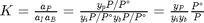
K = prod(yj.^nuj)
K =

    1.4359
end

% categories: optimization
% tags: Thermodynamics, reaction engineering
 . Recalling that we define
 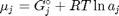 , and in the ideal gas limit,
  , and that
  . Since in this problem, P = 1 atm, this leads to the function
 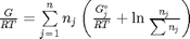 .
. where
where  is a vector of the moles of each species present in the mixture. CH4 C2H4 C2H2 CO2 CO O2 H2 H2O C2H6
 . Even though nearly all the ethane is consumed, we don't get the full yield of hydrogen. It appears that another equilibrium, one between CO, CO2, H2O and H2, may be limiting that, since the rest of the hydrogen is largely in the water. It is also of great importance that we have not said anything about reactions, i.e. how these products were formed. This is in stark contrast to
  . We can compute the Gibbs free energy of the reaction from the heats of formation of each species. Assuming these are the formation energies at 1000K, this is the reaction free energy at 1000K.
 where
where  is the chemical potential of species
  , and it is temperature and pressure dependent, and
  is the number of moles of species
  , where
  is the Gibbs energy in a standard state, and
  is the activity of species
  and stoichiometric coefficients:
  . Note that the reaction extent has units of moles.
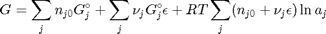
 . With these observations we rewrite the equation as:
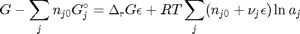
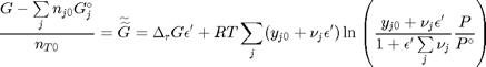
 . It is desirable to avoid this, so we now rescale the equation by the total initial moles present,
  and define a new variable
  , which is dimensionless. This leads to:
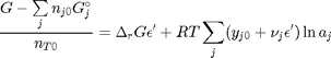
 is the initial mole fraction of species
  , where the numerator is the partial pressure of species
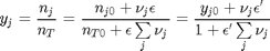
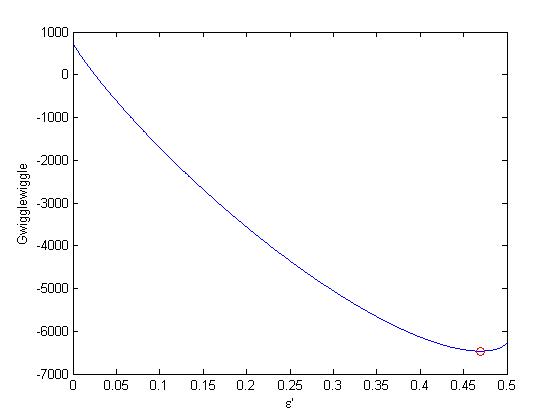
 . This additional scaling makes the quantities dimensionless, and makes the quantity have a magnitude of order unity, but otherwise has no effect on the shape of the graph.
 can be. Recall that
  , and that
  . Thus,
  , and the maximum value that
  where
where  . When there are multiple species, you need the smallest
  to avoid getting negative mole numbers.
 .
. . We can illustrate the conservation of mass with the following equation:
  . Where
  is the stoichiometric coefficient vector and
  is a column vector of molecular weights. For simplicity, we use pure isotope molecular weights, and not the isotope-weighted molecular weights.
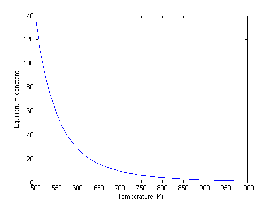
 in the temperature range of 500K to 1000K.
 and
and 


 , and
, and  is the temperature in Kelvin. We can use this data to calculate equilibrium constants in the following manner. First, we have heats of formation at standard state for each compound; for elements, these are zero by definition, and for non-elements, they have values available from the NIST webbook. There are also values for the absolute entropy at standard state. Then, we have an expression for the change in enthalpy from standard state as defined above, as well as the absolute entropy. From these we can derive the reaction enthalpy, free energy and entropy at standard state, as well as at other temperatures.
 .
. and
and 

 are the stoichiometric coefficients of each species, with appropriate sign for reactants and products, and
 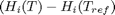 is precisely what is calculated for each species with the equations
 varies with temperature
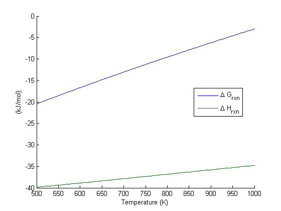
 be the extent of reaction, so that
  . For reactants,
  is negative, and for products,