Plane Poiseuille flow - BVP
August 11, 2011 at 04:49 PM | categories: odes | View Comments
Plane Poiseuille flow - BVP
in the pressure driven flow of a fluid with viscosity  between two stationary plates separated by distance
  and driven by a pressure drop
  , the governing equations on the velocity
  of the fluid are (assuming flow in the x-direction with the velocity varying only in the y-direction):

with boundary conditions  and
and  , i.e. the no-slip condition at the edges of the plate.
we convert this second order BVP to a system of ODEs by letting  ,
,  and then
  . This leads to:


with boundary conditions  and
and  .
.
for this problem we let the plate separation be d=0.1, the viscosity  , and
, and  .
.
function main
clc; close all; clear all;

d = 0.1; % plate thickness
we start by defining an initial grid to get the solution on
x = linspace(0,d);
Next, we use the bvpinit command to provide an initial guess using the guess function defined below
solinit = bvpinit(x,@guess);
we also need to define the ode function (see odefun below).
and a boundary condition function (see bcfun below).
now we can get the solution.
sol = bvp5c(@odefun,@bcfun,solinit)
sol =

    solver: 'bvp5c'
         x: [1x100 double]
         y: [2x100 double]
     idata: [1x1 struct]
     stats: [1x1 struct]
sol is a Matlab struct with fields. the x field contains the x-values of the solution as a row vector, the y field contains the solutions to the odes. Recall that U1 is the only solution we care about, as it is the original u(x) we were interested in.
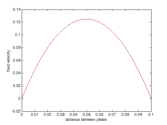
y = sol.x;
u1 = sol.y(1,:);
u2 = sol.y(2,:);
plot(y,u1); figure(gcf)
xlabel('distance between plates')
ylabel('fluid velocity')

% the analytical solution to this problem is known, and we can plot it on
% top of the numerical solution
mu = 1;
Pdrop = -100; % this is DeltaP/Deltax
u = -(Pdrop)*d^2/2/mu*(y/d-(y/d).^2);
hold on
plot(y,u,'r--')
As we would expect, the solutions agree, and show that the velocity profile is parabolic, with a maximum in the middle of the two plates. You can also see that the velocity at each boundary is zero, as required by the boundary conditions
function Uinit = guess(x)
% this is an initial guess of the solution. We need to provide a guess of
% what the function values of u1(y) and u2(y) are for a value of y. In some
% cases, this initial guess may affect the ability of the solver to get a
% solution. In this example, we guess that u1 and u2 are constants
U1 = 0.1;
U2 = 0;
Uinit = [U1; U2]; % we return a column vector

function dUdy = odefun(y,U)
% here we define our differential equations
u1 = U(1);
u2 = U(2);

mu = 1;
Pdrop = -100; % this is DeltaP/Deltax
du1dy = u2;
du2dy = 1/mu*Pdrop;
dUdy = [du1dy; du2dy];

function res = bcfun(U_0,U_d)
% this function defines the boundary conditions for each ode.
% we define the velocity at y=0 and y=d to be zero here. If the plates are
% moving, you would substitute the velocity of each plate for the zeros.
res = [0 - U_0(1);
       0 - U_d(1)];

% categories: ODEs
% tags: math, fluids

 and
and  . To solve this in Matlab, we need to convert the second order differential equation into a system of first order ODEs, and use the bvp5c command to get a numerical solution.
 . but the bvp5c syntax takes a lot to get used to.
 , and
, and  . That leads to
  and the following set of equations:

 and
and  . By inspection you can see that whatever value
  has, it will remain constant since the derivative of
 although Matlab does not print it this nicely!

 and
and  . This leads to:

 and
and  at
at  on a grid over the range of values for
  and
and  we are interested in. We will plot the derivatives as a vector at each (y1, y2) which will show us the initial direction from each point. We will examine the solutions over the range -2 < y1 < 8, and -2 < y2 < 2 for y2, and create a grid of 20x20 points.
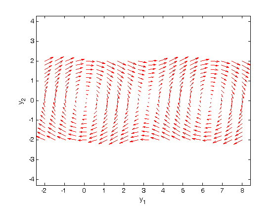
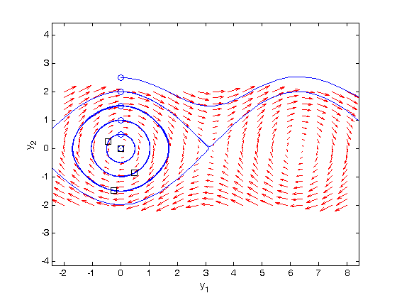
 to
to  . The y1 data in this case is not wrapped around to be in this range.
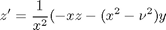
 comes up often in engineering problems such as heat transfer. The solutions to this equation are the Bessel functions. To solve this equation numerically, we must convert it to a system of first order ODEs. This can be done by letting
  and
and  and performing the change of variables:
 , the solution is known to be the Bessel function
  , which is represented in Matlab as besselj(0,x). The initial conditions for this problem are:
  and
and  .
. term, the ODEs are not defined at x=0.