Matlab in Chemical Engineering at CMU

Plane Poiseuille flow - BVP

August 11, 2011 at 04:49 PM | categories: odes | View Comments

Plane Poiseuille flow - BVP

in the pressure driven flow of a fluid with viscosity $\mu$ between two stationary plates separated by distance $d$ and driven by a pressure drop $\Delta P/\Delta x$ , the governing equations on the velocity $u$ of the fluid are (assuming flow in the x-direction with the velocity varying only in the y-direction):

$\frac{\Delta P}{\Delta x} = \mu \frac{d^2u}{dy^2}$

with boundary conditions $u(y=0) = 0$ and $u(y=d) = 0$ , i.e. the no-slip condition at the edges of the plate.

we convert this second order BVP to a system of ODEs by letting $u_1 = u$ , $u_2 = u_1'$ and then $u_2' = u_1''$ . This leads to:

$\frac{d u_1}{dy} = u_2$

$\frac{d u_2}{dy} = \frac{1}{\mu}\frac{\Delta P}{\Delta x}$

with boundary conditions $u_1(y=0) = 0$ and $u_1(y=d) = 0$ .

for this problem we let the plate separation be d=0.1, the viscosity $\mu = 1$ , and $\frac{\Delta P}{\Delta x} = -100$ .

function main

clc; close all; clear all;

d = 0.1; % plate thickness

we start by defining an initial grid to get the solution on

x = linspace(0,d);

Next, we use the bvpinit command to provide an initial guess using the guess function defined below

solinit = bvpinit(x,@guess);

we also need to define the ode function (see odefun below).

and a boundary condition function (see bcfun below).

now we can get the solution.

sol = bvp5c(@odefun,@bcfun,solinit)

sol = 

    solver: 'bvp5c'
         x: [1x100 double]
         y: [2x100 double]
     idata: [1x1 struct]
     stats: [1x1 struct]

sol is a Matlab struct with fields. the x field contains the x-values of the solution as a row vector, the y field contains the solutions to the odes. Recall that U1 is the only solution we care about, as it is the original u(x) we were interested in.

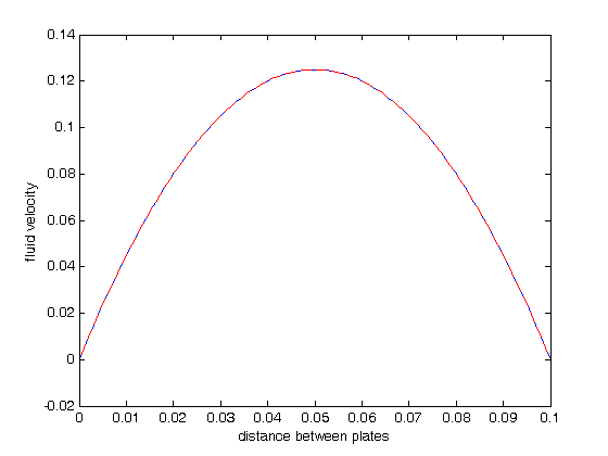
y = sol.x;
u1 = sol.y(1,:);
u2 = sol.y(2,:);
plot(y,u1); figure(gcf)
xlabel('distance between plates')
ylabel('fluid velocity')

% the analytical solution to this problem is known, and we can plot it on
% top of the numerical solution
mu = 1;
Pdrop = -100; % this is DeltaP/Deltax
u = -(Pdrop)*d^2/2/mu*(y/d-(y/d).^2);
hold on
plot(y,u,'r--')

As we would expect, the solutions agree, and show that the velocity profile is parabolic, with a maximum in the middle of the two plates. You can also see that the velocity at each boundary is zero, as required by the boundary conditions

function Uinit = guess(x)
% this is an initial guess of the solution. We need to provide a guess of
% what the function values of u1(y) and u2(y) are for a value of y. In some
% cases, this initial guess may affect the ability of the solver to get a
% solution. In this example, we guess that u1 and u2 are constants
U1 = 0.1;
U2 = 0;
Uinit = [U1; U2]; % we return a column vector

function dUdy = odefun(y,U)
% here we define our differential equations
u1 = U(1);
u2 = U(2);

mu = 1;
Pdrop = -100; % this is DeltaP/Deltax
du1dy = u2;
du2dy = 1/mu*Pdrop;
dUdy = [du1dy; du2dy];

function res = bcfun(U_0,U_d)
% this function defines the boundary conditions for each ode.
% we define the velocity at y=0 and y=d to be zero here. If the plates are
% moving, you would substitute the velocity of each plate for the zeros.
res = [0 - U_0(1);
       0 - U_d(1)];

% categories: ODEs
% tags: math, fluids