Sums, products and linear algebra notation - avoiding loops where possible
January 03, 2012 at 05:03 PM | categories: linear algebra | View Comments
Sums, products and linear algebra notation - avoiding loops where possible
John Kitchin
Today we examine some methods of linear algebra that allow us to avoid writing explicit loops in Matlab for some kinds of mathematical operations.
Contents
Consider the operation on two vectors  and
and  .
.

a = [1 2 3 4 5];
b = [3 6 8 9 10];
Old-fashioned way with a loop
We can compute this with a loop, where you initialize y, and then add the product of the ith elements of a and b to y in each iteration of the loop. This is known to be slow for large vectors
y = 0;
for i=1:length(a)
    y = y + a(i)*b(i);
end

y
y =

   125
dot notation
Matlab defines dot operators, so we can compute the element-wise product of  and
and  , and then use the builtin sum command to get the result.
y = sum(a.*b)
y =

   125
dot product
The operation above is formally the definition of a dot product. We can directly compute this in Matlab. Note that one vector must be transposed so that we have the right dimensions for legal matrix multiplication (one vector must be a row, and one must be column). It does not matter which order the multiplication is done as shown here.
y = a*b'

y = b*a'
y =

   125


y =

   125
Another example

This operation is like a weighted sum of squares.
w = [0.1 0.25 0.12 0.45 0.98];
x = [9 7 11 12 8];
Old-fashioned method with a loop
y = 0;
for i = 1:length(w)
    y = y + w(i)*x(i)^2;
end
y
y =

  162.3900
dot operator approach
We use parentheses to ensure that x is squared element-wise before the element-wise multiplication.
y = sum(w.*(x.^2))
y =

  162.3900
Linear algebra approach
The operation is mathematically equivalent to  when
when  is a row vector.
  is a diagonal matrix with the values of
  on the diagonal, and zeros everywhere else. The Matlab command diag creates this matrix conveniently.
y = x*diag(w)*x'
y =

  162.3900
Last example

This operation is like a weighted sum of products.
w = [0.1 0.25 0.12 0.45 0.98];
x = [9 7 11 12 8];
y = [2 5 3 8 0];
Old fashioned method with a loop
z = 0;
for i=1:length(w)
    z = z + w(i)*x(i)*y(i);
end
z
z =

   57.7100
dot notation
we use parentheses
z = sum(w.*x.*y)
z =

   57.7100
Linear algebra approach
Note that it does not matter what order the dot products are done in, just as it does not matter what order w(i)*x(i)*y(i) is multiplied in.
z = x*diag(w)*y'
z = y*diag(x)*w'
z = w*diag(y)*x'
z =

   57.7100


z =

   57.7100


z =

   57.7100
Summary
We showed examples of the following equalities between traditional sum notations and linear algebra

These relationships enable one to write the sums as a single line of Matlab code, which utilizes fast linear algebra subroutines, avoids the construction of slow loops, and reduces the opportunity for errors in the code. Admittedly, it introduces the opportunity for new types of errors, like using the wrong relationship, or linear algebra errors due to matrix size mismatches.
% categories: Linear Algebra
% tags: math
 that is the solution to the following set of equations:
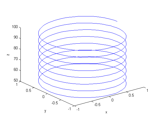
![$f(0,0,0) = [0,0, 100]$](http://matlab.cheme.cmu.edu/wp-content/uploads/2011/11/plot_cylindrical_ode_soln_eq521161.png) . There is nothing special about these equations; they describe a cork screw with constant radius. Solving the equations is simple; they are not coupled, and we simply integrate each equation with ode45. Plotting the solution is trickier, because we have to convert the solution from cylindrical coordinates to cartesian coordinates for plotting.
. There is nothing special about these equations; they describe a cork screw with constant radius. Solving the equations is simple; they are not coupled, and we simply integrate each equation with ode45. Plotting the solution is trickier, because we have to convert the solution from cylindrical coordinates to cartesian coordinates for plotting.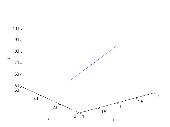
 , so that at
  we have a simpler problem we know how to solve, and at
  we have the original set of equations. Then, we derive a set of ODEs on how the solution changes with
  , which has two roots,
  and
and  . We will use the method of continuity to solve this equation to illustrate a few ideas. First, we introduce a new variable
  . For example, we could write
  . Now, when
  , with the solution
  . The question now is, how does
  change as
  changes with
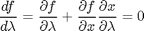
 and
and  analytically from our equation and solve for
  as
as
 and
and  .
.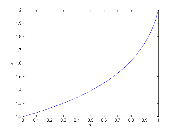
 into the equations in another way. We could try:
  , but this leads to an ODE that is singular at the initial starting point. Another approach is
  , but now the solution at
  is imaginary, and we don't have a way to integrate that! What we can do instead is add and subtract a number like this:
  . Now at
  , and we already know that
  is a solution. So, we create our ODE on
  with initial condition
  .
.
 , you find that 2 is a root, and learn nothing new. You could choose other values to add, e.g., if you chose to add and subtract 16, then you would find that one starting point leads to one root, and the other starting point leads to the other root. This method does not solve all problems associated with nonlinear root solving, namely, how many roots are there, and which one is "best"? But it does give a way to solve an equation where you have no idea what an initial guess should be. You can see, however, that just like you can get different answers from different initial guesses, here you can get different answers by setting up the equations differently.
 matrix
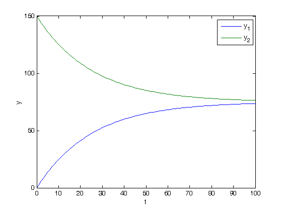
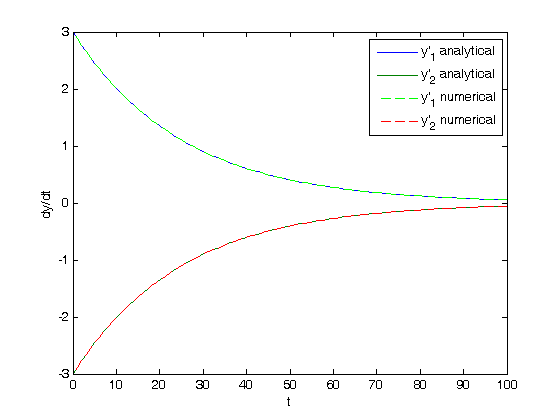
![$\left[\begin{array}{c}y'_1\\y'_2\end{array}\right] = \left[\begin{array}{cc} -0.02 & 0.02 \\ 0.02 & -0.02\end{array}\right] \left[\begin{array}{c}y_1\\y_2\end{array}\right]$](http://matlab.cheme.cmu.edu/wp-content/uploads/2011/10/const_coeff_coupled_eq84697.png)
![$\left[\begin{array}{c}y_1\\y_2\end{array}\right] = \left[\begin{array}{cc}v_1 & v_2\end{array}\right] \left[\begin{array}{cc} c_1 & 0 \\ 0 & c_2\end{array}\right] \exp\left(\left[\begin{array}{cc} \lambda_1 & 0 \\ 0 & \lambda_2\end{array}\right] \left[\begin{array}{c}t\\t\end{array}\right]\right)$](http://matlab.cheme.cmu.edu/wp-content/uploads/2011/10/const_coeff_coupled_eq32208.png)
![$\left[\begin{array}{cc} \lambda_1 & 0 \\ 0 & \lambda_2\end{array}\right]$](http://matlab.cheme.cmu.edu/wp-content/uploads/2011/10/const_coeff_coupled_eq06652.png) is a diagonal matrix of the eigenvalues of the constant coefficient matrix,
is a diagonal matrix of the eigenvalues of the constant coefficient matrix, ![$\left[\begin{array}{cc}v_1 & v_2\end{array}\right]$](http://matlab.cheme.cmu.edu/wp-content/uploads/2011/10/const_coeff_coupled_eq51102.png) is a matrix of eigenvectors where the
is a matrix of eigenvectors where the  column corresponds to the eigenvector of the
 ![$\left[\begin{array}{cc} c_1 & 0 \\ 0 & c_2\end{array}\right]$](http://matlab.cheme.cmu.edu/wp-content/uploads/2011/10/const_coeff_coupled_eq84783.png) is a matrix determined by the initial conditions.
is a matrix determined by the initial conditions. and
and  .
. matrix
 and
and  .
.
 . To approximate the integral, we need to divide the interval from
  to
to  into
into  intervals. The analytical answer is 2.0.