Controlling the exit concentration of a CSTR

| categories: miscellaneous | View Comments

Controlling the exit concentration of a CSTR

Controlling the exit concentration of a CSTR

John Kitchin

We examine how to model a CSTR with a controller that varies the volumetric flowrate to control the exit concentration. First we examine a case with no control, then with a simple controller, and then the response of the controller to a change in temperature which modifies the reaction rate.

function main
close all, clc, clear all

V = 100; % volume of CSTR
vo = 20; % volumetric flow rate
Cain = 2;
Ca0 = 2;
tspan = linspace(0,20,20*60); % this is the solution at every second.

    function dCadt = cstr(t,Ca)
        % A -> B
        ra = -0.1*Ca;
        dCadt =  Cain - Ca + ra*V/vo ;
    end

[t,Ca] = ode45(@cstr,tspan,Ca0);

subplot(2,1,1)
plot(t,Ca)
xlabel('Time')
ylabel('C_A')

subplot(2,1,2)
plot(tspan,vo,'b.')
xlabel('time')
ylabel('volumetric flow')

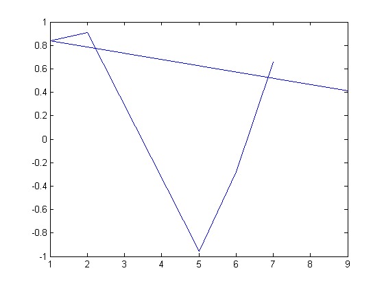
The reactor does not have the desired behavior; the exit concentration is too high. We could simply compute the flow rate required to get the desired exit concentration, but that will only work for this specific set of conditions. If the reactor gets hotter or colder, it will no longer have the desired exit concentration because the reaction rates will change.

Let's implement a controller to actively control the exit concentration by varying the volumetric flow. We will use a simple idea: if the exit concentration is not equal to the desired setpoint, we adjust the volumetric flow by an amount proportional to the difference. We call the proportionality the gain. The choice of the gain factor can have a major impact on the controller. If it is too low, it takes a long time for the system to respond, and if it is too high, the controller may actually be unstable. Here we use a gain that works ok, which we discovered by trial and error. There are ways to determine an optimal behavior that are beyond the scope of this post.

We choose an exit goal of 0.5 mol A/L, corresponding to a conversion of 0.75 for the inlet concentration.

    function vo_in = controller(t,Ca)
        % a simple proportional controller that adjusts  the volumetric
        % flow by an amount proportional to the deviation between the
        % desired and actual exit concentrations.

        setpoint = 0.5;  % desired exit concentration
        error = setpoint - Ca;

        gain = 0.5;
        vo = vo + gain*error;

        % We don't want to allow vo to be negative, and practically it
        % cannot be zero either, since then tau = infinity. Our pump is
        % also limited to a maximum volumetric flow of 40.
        if vo < 0.001;
            vo = 0.001
        elseif vo > 40
            vo = 40;
        end

        % let's plot the volumetric flow to see how it changes everytime
        % this function is called.
        subplot(2,1,2); hold on
        plot(t,vo,'b.')
        vo_in = vo;
    end

    function dCadt = controlled_cstr(t,Ca)
        % A -> B
        ra = -0.1*Ca;

        % the next line sets the volumetric flow.
        vo = controller(t,Ca);
        dCadt =  Cain - Ca + ra*V/vo ;
    end

tspan = linspace(20,40,20*60);
init = Ca(end); % start at the end of the last integration

[t2,Ca2] = ode45(@controlled_cstr,tspan,init);
subplot(2,1,1); hold on
plot(t2,Ca2,'r-')

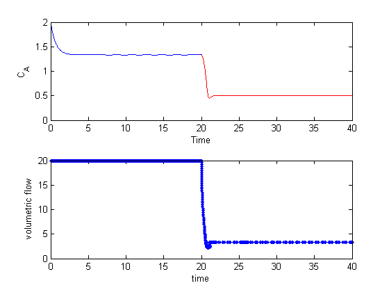
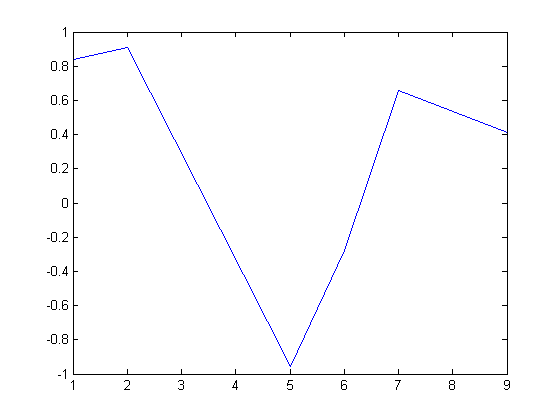
The controller quickly decreases the volumetric flowrate to increase the residence time, resulting in a decrease in exit concentration. Here you can see the gain is a little too high, because the controller overshoots and the exit concentration, and there are some excursions from the setpoint after that. Those are due to numerical errors in the ODE integration.

Now let's see how the controller responds to a temperature excursion. Suppose the reactor cools down, and the reaction rate is suddenly one half the rate it used to be. The exit concentration will rise, since the reactants are not reacting as fast. The controller should decrease the volumetric flowrate to increase the space time.

    function dCadt = controlled_cstr_temperature(t,Ca)
        % A -> B
        ra = -0.05*Ca;
        vo = controller(t,Ca);
        dCadt =  Cain - Ca + ra*V/vo ;
    end

tspan = linspace(40,60,20*60);
init = Ca2(end); % start at the end of the last integration

[t3,Ca3] = ode45(@controlled_cstr_temperature,tspan,init);

subplot(2,1,1); hold on
plot(t3,Ca3,'k-')

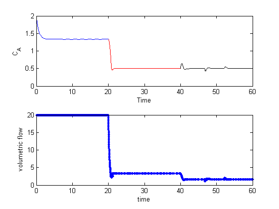
As expected, the concentration initially goes up, then the controller lowers the volumetric flowrate. Also note the controller was able to keep the exit concentration at the setpoint even though the rate of the reaction changed due to the temperature change. There are some notable small deviations from the setpoint near times 47 and 52. These are due to the ODE solver. If you examine the spacing of the points in the volumetric flow graph you will see they are not evenly spaced at 1 sec. That is because the volumetric flow is updated for every call to the ode function, not just at the solution points.

Now that I have tried this, it is clear this is not the best way to model the effect of a controller, because the ODE integrator does some funny things with the time steps. Sometimes the solver appears to take steps back in time to improve the accuracy of the solution, but that is not physically real, and the controller doesn't account for this non-physical behavior. That is why, for example there are excursions from the setpoint after an apparent steady state value is reached in the last example. Maybe this is why everyone uses Simulink for control problems!

end

% categories: Miscellaneous
% tags: control
% post_id = 1460; %delete this line to force new post;
% permaLink = http://matlab.cheme.cmu.edu/2011/11/13/control_cstr-m/;
Read and Post Comments

Unique entries in a vector

| categories: miscellaneous | View Comments

unique_entries

Contents

Unique entries in a vector

John Kitchin

It is surprising how often you need to know only the unique entries in a vector of entries. Matlab provides the unique` to solve these problems. The :command:`unique command returns the sorted unique entries in a vector.

a = [1 1 2 3 4 5 3 5]

unique(a)
a =

     1     1     2     3     4     5     3     5


ans =

     1     2     3     4     5

The unique command also works with cell arrays of strings.

a = {'a'
    'b'
    'abracadabra'
    'b'
    'c'
    'd'
    'b'}

unique(a)
a = 

    'a'
    'b'
    'abracadabra'
    'b'
    'c'
    'd'
    'b'


ans = 

    'a'
    'abracadabra'
    'b'
    'c'
    'd'

There is more!

The unique command has some other features too. check them out:

help unique
 UNIQUE Set unique.
    B = UNIQUE(A) for the array A returns the same values as in A but
    with no repetitions. B will also be sorted. A can be a cell array of
    strings.
 
    UNIQUE(A,'rows') for the matrix A returns the unique rows of A.
 
    [B,I,J] = UNIQUE(...) also returns index vectors I and J such
    that B = A(I) and A = B(J) (or B = A(I,:) and A = B(J,:)).
 
    [B,I,J] = UNIQUE(...,'first') returns the vector I to index the
    first occurrence of each unique value in A.  UNIQUE(...,'last'),
    the default, returns the vector I to index the last occurrence.
 
    See also UNION, INTERSECT, SETDIFF, SETXOR, ISMEMBER, SORT, ISSORTED.

    Overloaded methods:
       cell/unique
       dataset/unique
       RTW.unique
       categorical/unique

    Reference page in Help browser
       doc unique

'done'

% categories: Miscellaneous
ans =

done

Read and Post Comments

Sorting in Matlab

| categories: miscellaneous | View Comments

Sorting in Matlab

Sorting in Matlab

John Kitchin

Occasionally it is important to have sorted data. Matlab provides a sort command with a variety of behaviors that you can use, as well as other related commands.

Contents

Sorting a vector

a = [4 5 1 6 8 3 2]
a =

     4     5     1     6     8     3     2

b_ascending = sort(a)  % default is in ascending order
b_ascending =

     1     2     3     4     5     6     8

You can specify descending order like this

b_descending = sort(a,'descend')
b_descending =

     8     6     5     4     3     2     1

or you can use the command fliplr to reverse the vector sorted in ascending order.

fliplr(b_ascending)
ans =

     8     6     5     4     3     2     1

Sorting a matrix

If you have data organized in a matrix, you need to be aware of what sorting means. You can sort rows or columns!

a = [5 1 5 4 3
     0 7 1 2 3];

 sort(a)
ans =

     0     1     1     2     3
     5     7     5     4     3

sort works columnwise by default. If you wanted the rows sorted, you need:

sort(a,2)
ans =

     1     3     4     5     5
     0     1     2     3     7

How can you remember that? Indexing in Matlab is (row,column). This notation means sort along the columns. In other words, the row is fixed, and you sort along the columns.

Where would this ever come up? We use it in cmu.der.derc to ensure the x-values are in ascending order before we compute the derivative! It is also convenient to sort data before plotting it if you connect the datapoints by lines.

x = [9 1 2 5 6 7];
y = sin(x);

plot(x,y)

Note how the lines cross each other. That is visually distracting, and simply an artifact of the ordering of the points. We can use an extra feature of sort to sort x and y, so that x is sorted in ascending order, and we use the change in the order of x to get the corresponding changes in y. This is a handy trick!

[X I] = sort(x);
Y = y(I);
plot(X,Y)
'done'

% categories: Miscellaneous
ans =

done

Read and Post Comments

Interacting with labeled data points

| categories: plotting | View Comments

using_gname

Contents

Interacting with labeled data points

John Kitchin

Matlab has a lot of capabilities for interacting graphically with data sets. Let's consider a dataset that contains ratings for different cities in different categories, such as health and climate. We suppose there could be a correlation between these two ratings and we want to check that.

Watch the video: http://screencast.com/t/PeIzxp3n

clear ; close all; clc
load cities % Matlab example data set

extract data for easy plotting

climate = ratings(:,1);
health  = ratings(:,3);
plot(climate,health,'ro')
xlabel('Climate rating')
ylabel('Health rating')

Identifying each data point.

gname(names)


% categories: plotting

% post_id = 1431; %delete this line to force new post;
% permaLink = http://matlab.cheme.cmu.edu/2011/11/11/interacting-with-labeled-data-points/;
Read and Post Comments

plot the solution to an ODE in cylindrical coordinates

| categories: odes, plotting | View Comments

plot the solution to an ODE in cylindrical coordinates

plot the solution to an ODE in cylindrical coordinates

John Kitchin

Matlab provides pretty comprehensive support to plot functions in cartesian coordinates. There is no direct support to plot in cylindrical coordinates, however. In this post, we learn how to solve an ODE in cylindrical coordinates, and to plot the solution in cylindrical coordinates.

We want the function $f(\rho,\theta,z)$ 
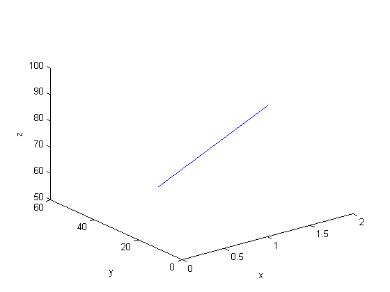
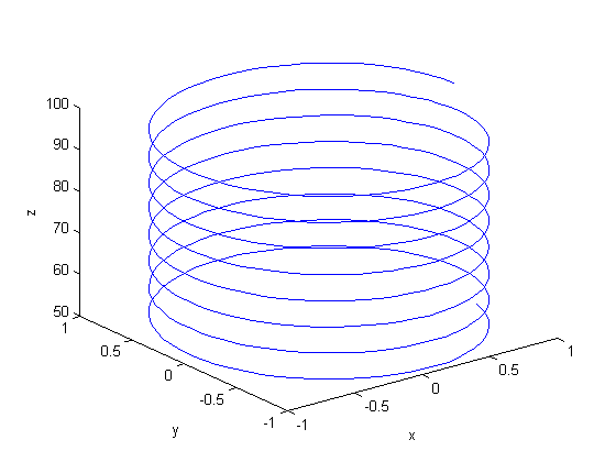
that is the solution to the following set of equations:

Contents

$$\begin{array}{l} \frac{d\rho}{dt} = 0\\
\frac{d\theta}{dt} = 1 \\
\frac{dz}{dt} = -1
\end{array}$$

with initial conditions $f(0,0,0) = [0,0, 100]$. There is nothing special about these equations; they describe a cork screw with constant radius. Solving the equations is simple; they are not coupled, and we simply integrate each equation with ode45. Plotting the solution is trickier, because we have to convert the solution from cylindrical coordinates to cartesian coordinates for plotting.

function main
    function dfdt = cylindrical_ode(t,F)
        rho = F(1);
        theta = F(2);
        z = F(3);

        drhodt = 0; % constant radius
        dthetadt = 1; % constant angular velocity
        dzdt = -1; % constant dropping velocity
        dfdt = [drhodt; dthetadt; dzdt];
    end

rho0 = 1;
theta0 = 0;
z0 = 100;

tspan = linspace(0,50,500);
[t,f] = ode45(@cylindrical_ode,tspan,[rho0 theta0 z0]);

rho = f(:,1);
theta = f(:,2);
z = f(:,3);

plot3(rho,theta,z)
xlabel('x')
ylabel('y')
zlabel('z')

This is not a cork screw at all! The problem is that plot3 expects cartesian coordinates, but we plotted cylindrical coordinates. To use the plot3 function we must convert the cylindrical coordinates to cartesian coordinates. Matlab provides a simple utility for doing that.

Convert the cylindrical coordinates to cartesian coordinates

[X Y Z] = pol2cart(theta,rho,z);

plot3(X,Y,Z)
xlabel('x')
ylabel('y')
zlabel('z')

That is the corkscrew we were expecting! The axes are still the x,y,z axes. It doesn't make sense to label them anything else.

end

% categories: ODEs, plotting
% tags: math
Read and Post Comments

« Previous Page -- Next Page »