Sums, products and linear algebra notation - avoiding loops where possible

| categories: linear algebra | View Comments

Sums, products and linear algebra notation - avoiding loops where possible

Sums, products and linear algebra notation - avoiding loops where possible

John Kitchin

Today we examine some methods of linear algebra that allow us to avoid writing explicit loops in Matlab for some kinds of mathematical operations.

Contents

Consider the operation on two vectors $\bf{a}$ and $\bf{b}$.

$$y=\sum\limits_{i=1}^n a_ib_i$$

a = [1 2 3 4 5];
b = [3 6 8 9 10];

Old-fashioned way with a loop

We can compute this with a loop, where you initialize y, and then add the product of the ith elements of a and b to y in each iteration of the loop. This is known to be slow for large vectors

y = 0;
for i=1:length(a)
    y = y + a(i)*b(i);
end

y
y =

   125

dot notation

Matlab defines dot operators, so we can compute the element-wise product of $\bf{a}$ and $\bf{b}$, and then use the builtin sum command to get the result.

y = sum(a.*b)
y =

   125

dot product

The operation above is formally the definition of a dot product. We can directly compute this in Matlab. Note that one vector must be transposed so that we have the right dimensions for legal matrix multiplication (one vector must be a row, and one must be column). It does not matter which order the multiplication is done as shown here.

y = a*b'

y = b*a'
y =

   125


y =

   125

Another example

$$y=\sum\limits_{i=1}^n w_ix_i^2$$

This operation is like a weighted sum of squares.

w = [0.1 0.25 0.12 0.45 0.98];
x = [9 7 11 12 8];

Old-fashioned method with a loop

y = 0;
for i = 1:length(w)
    y = y + w(i)*x(i)^2;
end
y
y =

  162.3900

dot operator approach

We use parentheses to ensure that x is squared element-wise before the element-wise multiplication.

y = sum(w.*(x.^2))
y =

  162.3900

Linear algebra approach

The operation is mathematically equivalent to $y = \bf{x}\bf{D_w}\bf{x^T}$ when $\bf{x}$ is a row vector. $\bf{D_w}$ is a diagonal matrix with the values of $\bf{w}$ on the diagonal, and zeros everywhere else. The Matlab command diag creates this matrix conveniently.

y = x*diag(w)*x'
y =

  162.3900

Last example

$$z=\sum\limits_{i=1}^n w_i x_i y_i$$

This operation is like a weighted sum of products.

w = [0.1 0.25 0.12 0.45 0.98];
x = [9 7 11 12 8];
y = [2 5 3 8 0];

Old fashioned method with a loop

z = 0;
for i=1:length(w)
    z = z + w(i)*x(i)*y(i);
end
z
z =

   57.7100

dot notation

we use parentheses

z = sum(w.*x.*y)
z =

   57.7100

Linear algebra approach

Note that it does not matter what order the dot products are done in, just as it does not matter what order w(i)*x(i)*y(i) is multiplied in.

z = x*diag(w)*y'
z = y*diag(x)*w'
z = w*diag(y)*x'
z =

   57.7100


z =

   57.7100


z =

   57.7100

Summary

We showed examples of the following equalities between traditional sum notations and linear algebra

$$\bf{a}\bf{b}=\sum\limits_{i=1}^n a_ib_i$$

$$\bf{x}\bf{D_w}\bf{x^T}=\sum\limits_{i=1}^n w_ix_i^2$$

$$\bf{x}\bf{D_w}\bf{y^T}=\sum\limits_{i=1}^n w_i x_i y_i$$

These relationships enable one to write the sums as a single line of Matlab code, which utilizes fast linear algebra subroutines, avoids the construction of slow loops, and reduces the opportunity for errors in the code. Admittedly, it introduces the opportunity for new types of errors, like using the wrong relationship, or linear algebra errors due to matrix size mismatches.

% categories: Linear Algebra
% tags: math
Read and Post Comments

Linear algebra approaches to solving systems of constant coefficient ODEs

| categories: linear algebra, odes | View Comments

const_coeff_coupled

Contents

Linear algebra approaches to solving systems of constant coefficient ODEs

John Kitchin

Today we consider how to solve a system of first order, constant coefficient ordinary differential equations using linear algebra. These equations could be solved numerically, but in this case there are analytical solutions that can be derived. The equations we will solve are:

$y'_1 = -0.02 y_1 + 0.02 y_2$

$y'_2 = 0.02 y_1 - 0.02 y_2$

We can express this set of equations in matrix form as: $\left[\begin{array}{c}y'_1\\y'_2\end{array}\right] = \left[\begin{array}{cc} -0.02 & 0.02 \\ 0.02 & -0.02\end{array}\right] \left[\begin{array}{c}y_1\\y_2\end{array}\right]$

The general solution to this set of equations is

$\left[\begin{array}{c}y_1\\y_2\end{array}\right] = \left[\begin{array}{cc}v_1 & v_2\end{array}\right] \left[\begin{array}{cc} c_1 & 0 \\ 0 & c_2\end{array}\right] \exp\left(\left[\begin{array}{cc} \lambda_1 & 0 \\ 0 & \lambda_2\end{array}\right] \left[\begin{array}{c}t\\t\end{array}\right]\right)$

where $\left[\begin{array}{cc} \lambda_1 & 0 \\ 0 & \lambda_2\end{array}\right]$ is a diagonal matrix of the eigenvalues of the constant coefficient matrix, $\left[\begin{array}{cc}v_1 & v_2\end{array}\right]$ is a matrix of eigenvectors where the $i^{th}$ column corresponds to the eigenvector of the $i^{th}$ eigenvalue, and $\left[\begin{array}{cc} c_1 & 0 \\ 0 & c_2\end{array}\right]$ is a matrix determined by the initial conditions.

In this example, we evaluate the solution using linear algebra. The initial conditions we will consider are $y_1(0)=0$ and $y_2(0)=150$.

close all
A = [-0.02 0.02;
    0.02 -0.02];

get the eigenvalues and eigenvectors of the A matrix

[V,D] = eig(A)
V =

    0.7071    0.7071
   -0.7071    0.7071


D =

   -0.0400         0
         0         0

V is a matrix of the eigenvectors, with each column being an eigenvector. Note that the eigenvectors are normalized so their length equals one. D is a diagonal matrix of eigenvalues.

Compute the $c$ matrix

V*c = Y0

We can solve this equation easily with the \ operator. As written, c will be a vector, but we need it in the form of a diagonal matrix, so we wrap the solution in the diag command.

Y0 = [0; 150]; % initial conditions
c = diag(V\Y0)
c =

 -106.0660         0
         0  106.0660

Constructing the solution

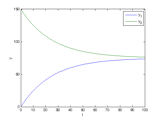
We will create a vector of time values, and stack them for each solution, $y_1(t)$ and $Y_2(t)$.

t = linspace(0,100);
T = [t;t];

y = V*c*exp(D*T);
plot(t,y)
xlabel('t')
ylabel('y')
legend 'y_1' 'y_2'

Verifying the solution

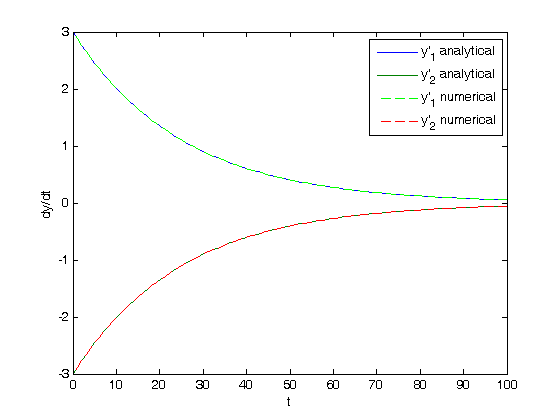
One way we can verify the solution is to analytically compute the derivatives from the differential equations, and then compare those derivatives to numerically evaluated derivatives from the solutions.

yp = A*y; % analytical derivatives

% numerically evaluated derivatves
yp1 = cmu.der.derc(t,y(1,:));
yp2 = cmu.der.derc(t,y(2,:));

plot(t,yp,t,yp1,'g--',t,yp2,'r--')
legend 'y''_1 analytical' 'y''_2 analytical' 'y''_1 numerical' 'y''_2 numerical'
xlabel('t')
ylabel('dy/dt')

What you can see here is that the analytical derivatives are visually equivalent to the numerical derivatives of the solution we derived.

'done'
% categories: ODEs, linear algebra
% tags: math
ans =

done

Read and Post Comments

Determining linear independence of a set of vectors

| categories: linear algebra | View Comments

Determining linear independence of a set of vectors

Determining linear independence of a set of vectors

Occasionally we have a set of vectors and we need to determine whether the vectors are linearly independent of each other. This may be necessary to determine if the vectors form a basis, or to determine how many independent equations there are, or to determine how many independent reactions there are.

Reference: Kreysig, Advanced Engineering Mathematics, sec. 7.4

Contents

Problem set 7.4 - #15

v1 = [6 0 3 1 4 2];
v2 = [0 -1 2 7 0 5];
v3 = [12 3 0 -19 8 -11];

R = rank([v1; v2; v3])
[rows, ~] = size([v1; v2; v3])
% note the ~ in the output indicates we do not care what the value is.

% the number of rows is greater than the rank, so these vectors are not
% independent. Let's demonstrate that one vector can be defined as a linear
% combination of the other two vectors. Mathematically we represent this
% as:
%
% $x_1 \mathit{v1} + x_2 \mathit{v2} = v3%
%
% or
%
% [x_1 x_2][v1; v2] = v3
%
% this is not the usual linear algebra form of Ax = b. To get there, we
% transpose each side of the equation to get:
%
% [v1.' v2.'][x_1; x_2] = v3'
%
% which is the form Ax = b. In Matlab we solve that as x = A\b (
R =

     2


rows =

     3

x = [v1.' v2.']\v3.'

x(1)*v1 + x(2)*v2
v3
% you can see that v3 = 2v1 - 3v2, illustrating that v3 is not linearly
% independent of v1 and v2.
x =

    2.0000
   -3.0000


ans =

   12.0000    3.0000    0.0000  -19.0000    8.0000  -11.0000


v3 =

    12     3     0   -19     8   -11

Problem set 7.4 #17

v1 = [0.2 1.2 5.3 2.8 1.6];
v2 = [4.3 3.4 0.9 2.0 -4.3];

rank([v1; v2])
% the rank is equal to the number of rows, so these vectors are linearly
% independent. You could also see that by inspection since the signs of the
% last element are different. there is no way to convert v1 to v2 by simple
% scaling.
ans =

     2

Near deficient rank

the rank command roughly works in the following way: the matrix is converted to a reduced row echelon form, and then the number of rows that are not all equal to zero are counted. Matlab uses a tolerance to determine what is equal to zero. If there is uncertainty in the numbers, you may have to define what zero is, e.g. if the absolute value of a number is less than 1e-5, you may consider that close enough to be zero. The default tolerance is usually very small, of order 1e-15.

A = [[1 2 3];
    [0 2 3];
    [0 0 1e-6]];

rank(A)
% matlab considers this matrix to have a full rank of 3 because the default
% tolerance in this case is 2.7e-15.
ans =

     3

rank with tolerance

If we believe that any number less than 1e-5 is practically equivalent to zero, we can use that information to compute the rank like this.

tolerance = 1e-5;
rank(A,tolerance)
% now the A matrix has a rank of only 2.
ans =

     2

Application to independent chemical reactions.

reference: Exercise 2.4 in Chemical Reactor Analysis and Design Fundamentals by Rawlings and Ekerdt.

The following reactions are proposed in the hydrogenation of bromine:

Let this be our species vector: v = [H2 H Br2 Br HBr]^T

the reactions are then defined by M*v where M is a stoichometric matrix in which each row represents a reaction with negative stoichiometric coefficients for reactants, and positive stoichiometric coefficients for products. A stoichiometric coefficient of 0 is used for species not participating in the reaction.

%    [H2  H Br2 Br HBr]
M = [[-1  0 -1  0  2];  % H2 + Br2 == 2HBR
     [ 0  0 -1  2  0];  % Br2 == 2Br
     [-1  1  0 -1  1];  % Br + H2 == HBr + H
     [ 0 -1 -1  1  1];  % H + Br2 == HBr + Br
     [ 1 -1  0  1  -1];  % H + HBr == H2 + Br
     [ 0  0  1 -2  0]]; % 2Br == Br2

rank(M)

% 6 reactions are given, but the rank of the matrix is only 3. so there
% are only four independent reactions. You can see that reaction 6 is just
% the opposite of reaction 2, so it is clearly not independent. Also,
% reactions 3 and 5 are just the reverse of each other, so one of them can
% also be eliminated. finally, reaction 4 is equal to reaction 1 minus
% reaction 3.
ans =

     3

choosing independent reactions

We can identify independent reactions by examining the reduced row echelon form of the matrix where the reactions are in the columns rather than rows. That is simply the transpose of the M matrix above. The columns with leading ones correspond to the reactions that can form a basis, i.e. the independent reactions.

rref(M')
% this shows columns 1,2,3 have leading ones, indicating the corresponding
% reactions are a suitable basis for all the reactions. If that is true,
% then we should be able to find solutions to the following linear
% equation: basis*x_i = reaction_i
ans =

     1     0     0     1     0     0
     0     1     0     0     0    -1
     0     0     1    -1    -1     0
     0     0     0     0     0     0
     0     0     0     0     0     0

basis = transpose(M(1:3,:)); % this is rows 1-3 of the M matrix

reaction_4 = M(4,:).';
reaction_5 = M(5,:).';
reaction_6 = M(6,:).';

x_4 = basis\reaction_4
x_5 = basis\reaction_5
x_6 = basis\reaction_6

% x_4, x_5 and x_6 are all integers, which means reactions 4, 5 and 6 are
% linear combinations of reactions 1, 2 and 3. As pointed out above, x_4
% shows reaction 4 to be reaction 1 - reaction 3; x_5 shows reaction 5 is
% -reaction 3; and x_6 shows reaction 6 is minus reaction 4.
x_4 =

    1.0000
    0.0000
   -1.0000


x_5 =

   -0.0000
    0.0000
   -1.0000


x_6 =

   -0.0000
   -1.0000
    0.0000

lets also demonstrate that reaction 1 is not a linear combination of reactions 2 and 3.

reaction_1 = M(1,:).';
x_1 = basis\reaction_1
% you can see the coefficients for reactions 2 and 3 are equal to zero,
% indicating reaction 1 is linearly independent of reactions 2 and 3.
x_1 =

    1.0000
    0.0000
    0.0000

Related posts

transposition rules

solving linear equations

% categories: Linear algebra
% tags: math, reaction engineering

% post_id = 640; %delete this line to force new post;
Read and Post Comments

Solving linear equations

| categories: linear algebra | View Comments

kreyszig_7_3

Contents

Solving linear equations

Given these equations, find [x1; x2; x3].

$x_1 - x_2 + x_3 = 0$

$10 x_2 + 25 x_3 = 90$

$20 x_1 + 10 x_2 = 80$

reference: Kreysig, Advanced Engineering Mathematics, 9th ed. Sec. 7.3

When solving linear equations, it is convenient to express the equations in matrix form:

A = [[1 -1 1];
    [0 10 25];
    [20 10 0]]

b = [0; 90; 80]  % b is a column vector
A =

     1    -1     1
     0    10    25
    20    10     0


b =

     0
    90
    80

making the augmented matrix

Awiggle = [A b]
Awiggle =

     1    -1     1     0
     0    10    25    90
    20    10     0    80

get the reduced row echelon form

rref(Awiggle)
ans =

     1     0     0     2
     0     1     0     4
     0     0     1     2

by inspection the solution is:

$x_1=2$

$x_2=4$

$x_3=2$

Let's test that out.

testing the solution

x = [2;4;2]
A*x
b
% you can see that A*x = b
x =

     2
     4
     2


ans =

     0
    90
    80


b =

     0
    90
    80

The shortcut way to solve this problem in Matlab with notation.

the backslash operator solves the equation Ax=b. Note that when there are more equations than unknowns

x = A\b
x =

    2.0000
    4.0000
    2.0000

linsolve function

x = linsolve(A,b)
x =

    2.0000
    4.0000
    2.0000

Not recommended solution methods

You may recall that a solution to

$\mathbf{A}\mathit{x} = \mathit{b}$

is:

$\mathit{x} = \mathbf{A}^{-1}\mathit{b}$

x = inv(A)*b

% while mathematically correct, computing the inverse of a matrix is
% computationally inefficient, and not recommended most of the time.
x =

    2.0000
    4.0000
    2.0000

What if no solution exists?

The following equations have no solution:

$3x_1 + 2x_2 + x_3 = 3$

$2x_1 + x_2 + x_3 = 0$

$6x_1 + 2x_2 + 4x_3 = 6$

A = [[3 2 1];
    [2 1 1];
    [6 2 4]]

b = [3; 0; 6]
A =

     3     2     1
     2     1     1
     6     2     4


b =

     3
     0
     6

how do you know no solution exists?

rref([A b])
% the last line of this matrix states that 0 = 1. That is not true, which
% means there is no solution.
ans =

     1     0     1     0
     0     1    -1     0
     0     0     0     1

Matlab gives you a solution anyway! and a warning.

x = A\b


% categories: Linear algebra
Warning: Matrix is close to singular or badly scaled.
         Results may be inaccurate. RCOND = 3.364312e-018. 

x =

  1.0e+016 *

    1.8014
   -1.8014
   -1.8014

Read and Post Comments

Illustrating matrix transpose rules in matrix multiplication

| categories: linear algebra | View Comments

Illustrating matrix transpose rules in matrix multiplication

Illustrating matrix transpose rules in matrix multiplication

John Kitchin

Contents

Rules for transposition

Here are the four rules for matrix multiplication and transposition

1. $(\mathbf{A}^T)^T = \mathbf{A}$

2. $(\mathbf{A}+\mathbf{B})^T = \mathbf{A}^T+\mathbf{B}^T$

3. $(\mathit{c}\mathbf{A})^T = \mathit{c}\mathbf{A}^T$

4. $(\mathbf{AB})^T = \mathbf{B}^T\mathbf{A}^T$

reference: Chapter 7.2 in Advanced Engineering Mathematics, 9th edition. by E. Kreyszig.

The transpose in Matlab

there are two ways to get the transpose of a matrix: with a notation, and with a function

A = [[5 -8 1];
    [4 0 0]]
A =

     5    -8     1
     4     0     0

function

transpose(A)
ans =

     5     4
    -8     0
     1     0

notation

A.'

% note, these functions only provide the non-conjugate transpose. If your
% matrices are complex, then you want the ctranspose function, or the
% notation A' (no dot before the apostrophe). For real matrices there is no
% difference between them.

% below we illustrate each rule using the different ways to get the
% transpose.
ans =

     5     4
    -8     0
     1     0

Rule 1

m1 = (A.').'
A

all(all(m1 == A)) % if this equals 1, then the two matrices are equal
m1 =

     5    -8     1
     4     0     0


A =

     5    -8     1
     4     0     0


ans =

     1

Rule 2

B = [[3 4 5];
    [1 2 3]];
m1 = transpose(A+B)
m2 = transpose(A) + transpose(B)

all(all(m1 == m2)) % if this equals 1, then the two matrices are equal
m1 =

     8     5
    -4     2
     6     3


m2 =

     8     5
    -4     2
     6     3


ans =

     1

Rule 3

c = 2.1;
m1 = transpose(c*A)
m2 = c*transpose(A)

all(all(m1 == m2)) % if this equals 1, then the two matrices are equal
m1 =

   10.5000    8.4000
  -16.8000         0
    2.1000         0


m2 =

   10.5000    8.4000
  -16.8000         0
    2.1000         0


ans =

     1

Rule 4

B = [[0 2];
    [1 2];
    [6 7]]

m1 = (A*B).'
m2 = B.'*A.'

all(all(m1 == m2)) % if this equals 1, then the two matrices are equal
B =

     0     2
     1     2
     6     7


m1 =

    -2     0
     1     8


m2 =

    -2     0
     1     8


ans =

     1

m3 = A.'*B.'
% you can see m3 has a different shape than m1, so there is no way they can
% be equal.
m3 =

     8    13    58
     0    -8   -48
     0     1     6

% categories: Linear algebra
% tags: math
% post_id = 552; %delete this line to force new post;
Read and Post Comments