Matlab in Chemical Engineering at CMU

Contents

Phase portraits of a system of ODEs

adapted from http://www-users.math.umd.edu/~tvp/246/matlabode2.html

clear all; close all; clc

Problem setup

An undamped pendulum with no driving force is described by

We reduce this to standard matlab form of a system of first order ODEs by letting and . This leads to:

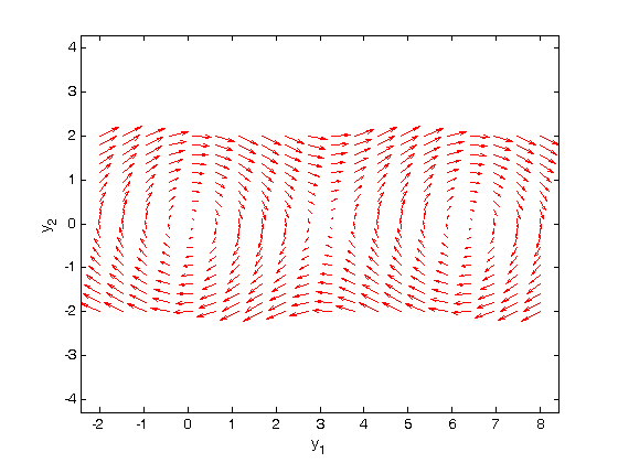
The phase portrait is a plot of a vector field which qualitatively shows how the solutions to these equations will go from a given starting point. here is our definition of the differential equations:

f = @(t,Y) [Y(2); -sin(Y(1))];

To generate the phase portrait, we need to compute the derivatives and at on a grid over the range of values for and we are interested in. We will plot the derivatives as a vector at each (y1, y2) which will show us the initial direction from each point. We will examine the solutions over the range -2 < y1 < 8, and -2 < y2 < 2 for y2, and create a grid of 20x20 points.

y1 = linspace(-2,8,20);
y2 = linspace(-2,2,20);

% creates two matrices one for all the x-values on the grid, and one for
% all the y-values on the grid. Note that x and y are matrices of the same
% size and shape, in this case 20 rows and 20 columns
[x,y] = meshgrid(y1,y2);
size(x)
size(y)

ans =

    20    20


ans =

    20    20

computing the vector field

we need to generate two matrices, u and v. u will contain the value of y1' at each x and y position, while v will contain the value of y2' at each x and y position of our grid.

we preallocate the arrays so they have the right size and shape

u = zeros(size(x));
v = zeros(size(x));

% we can use a single loop over each element to compute the derivatives at
% each point (y1, y2)
t=0; % we want the derivatives at each point at t=0, i.e. the starting time
for i = 1:numel(x)
    Yprime = f(t,[x(i); y(i)]);
    u(i) = Yprime(1);
    v(i) = Yprime(2);
end

now we use the quiver command to plot our vector field

quiver(x,y,u,v,'r'); figure(gcf)
xlabel('y_1')
ylabel('y_2')
axis tight equal;

Plotting solutions on the vector field

Let's plot a few solutions on the vector field. We will consider the solutions where y1(0)=0, and values of y2(0) = [0 0.5 1 1.5 2 2.5], in otherwords we start the pendulum at an angle of zero, with some angular velocity.

hold on
for y20 = [0 0.5 1 1.5 2 2.5]
    [ts,ys] = ode45(f,[0,50],[0;y20]);
    plot(ys(:,1),ys(:,2))
    plot(ys(1,1),ys(1,2),'bo') % starting point
    plot(ys(end,1),ys(end,2),'ks') % ending point
end
hold off

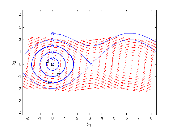
what do these figures mean? For starting points near the origin, and small velocities, the pendulum goes into a stable limit cycle. For others, the trajectory appears to fly off into y1 space. Recall that y1 is an angle that has values from to . The y1 data in this case is not wrapped around to be in this range.

'done'


% categories: ODEs
% tags: math
% post_id = 799; %delete this line to force new post;

ans =

done

Published with MATLAB® 7.10