plot the solution to an ODE in cylindrical coordinates
November 09, 2011 at 12:20 AM | categories: odes, plotting | View Comments
plot the solution to an ODE in cylindrical coordinates
John Kitchin
Matlab provides pretty comprehensive support to plot functions in cartesian coordinates. There is no direct support to plot in cylindrical coordinates, however. In this post, we learn how to solve an ODE in cylindrical coordinates, and to plot the solution in cylindrical coordinates.
We want the function  that is the solution to the following set of equations:
Contents

with initial conditions ![$f(0,0,0) = [0,0, 100]$](http://matlab.cheme.cmu.edu/wp-content/uploads/2011/11/plot_cylindrical_ode_soln_eq521161.png) . There is nothing special about these equations; they describe a cork screw with constant radius. Solving the equations is simple; they are not coupled, and we simply integrate each equation with ode45. Plotting the solution is trickier, because we have to convert the solution from cylindrical coordinates to cartesian coordinates for plotting.
. There is nothing special about these equations; they describe a cork screw with constant radius. Solving the equations is simple; they are not coupled, and we simply integrate each equation with ode45. Plotting the solution is trickier, because we have to convert the solution from cylindrical coordinates to cartesian coordinates for plotting.
function main
    function dfdt = cylindrical_ode(t,F)
        rho = F(1);
        theta = F(2);
        z = F(3);

        drhodt = 0; % constant radius
        dthetadt = 1; % constant angular velocity
        dzdt = -1; % constant dropping velocity
        dfdt = [drhodt; dthetadt; dzdt];
    end

rho0 = 1;
theta0 = 0;
z0 = 100;

tspan = linspace(0,50,500);
[t,f] = ode45(@cylindrical_ode,tspan,[rho0 theta0 z0]);

rho = f(:,1);
theta = f(:,2);
z = f(:,3);

plot3(rho,theta,z)
xlabel('x')
ylabel('y')
zlabel('z')
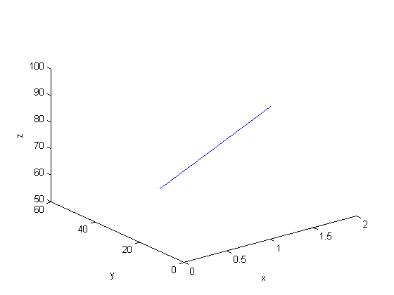
This is not a cork screw at all! The problem is that plot3 expects cartesian coordinates, but we plotted cylindrical coordinates. To use the plot3 function we must convert the cylindrical coordinates to cartesian coordinates. Matlab provides a simple utility for doing that.
Convert the cylindrical coordinates to cartesian coordinates
[X Y Z] = pol2cart(theta,rho,z);

plot3(X,Y,Z)
xlabel('x')
ylabel('y')
zlabel('z')
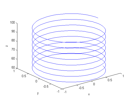
That is the corkscrew we were expecting! The axes are still the x,y,z axes. It doesn't make sense to label them anything else.
end

% categories: ODEs, plotting
% tags: math
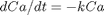 for multiple values of
  . Here we use a trick to pass a parameter to an ODE through the initial conditions. We expand the ode function definition to include this parameter, and set its derivative to zero, effectively making it a constant.
 value decays faster.
 matrix
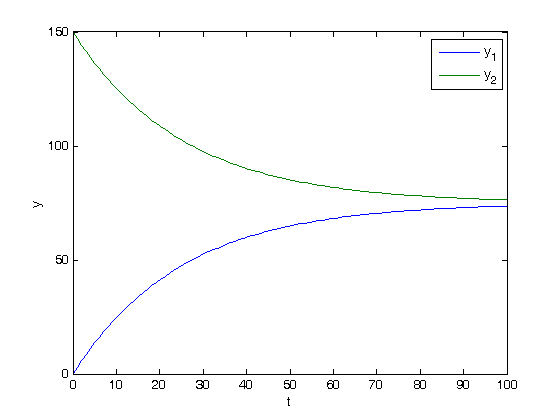
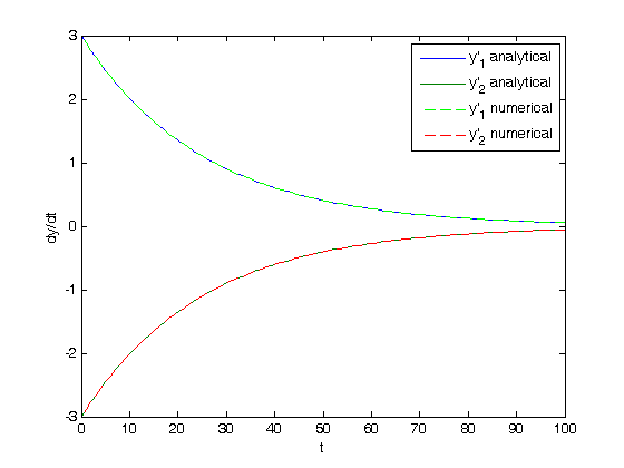
![$\left[\begin{array}{c}y'_1\\y'_2\end{array}\right] = \left[\begin{array}{cc} -0.02 & 0.02 \\ 0.02 & -0.02\end{array}\right] \left[\begin{array}{c}y_1\\y_2\end{array}\right]$](http://matlab.cheme.cmu.edu/wp-content/uploads/2011/10/const_coeff_coupled_eq84697.png)
![$\left[\begin{array}{c}y_1\\y_2\end{array}\right] = \left[\begin{array}{cc}v_1 & v_2\end{array}\right] \left[\begin{array}{cc} c_1 & 0 \\ 0 & c_2\end{array}\right] \exp\left(\left[\begin{array}{cc} \lambda_1 & 0 \\ 0 & \lambda_2\end{array}\right] \left[\begin{array}{c}t\\t\end{array}\right]\right)$](http://matlab.cheme.cmu.edu/wp-content/uploads/2011/10/const_coeff_coupled_eq32208.png)
![$\left[\begin{array}{cc} \lambda_1 & 0 \\ 0 & \lambda_2\end{array}\right]$](http://matlab.cheme.cmu.edu/wp-content/uploads/2011/10/const_coeff_coupled_eq06652.png) is a diagonal matrix of the eigenvalues of the constant coefficient matrix,
is a diagonal matrix of the eigenvalues of the constant coefficient matrix, ![$\left[\begin{array}{cc}v_1 & v_2\end{array}\right]$](http://matlab.cheme.cmu.edu/wp-content/uploads/2011/10/const_coeff_coupled_eq51102.png) is a matrix of eigenvectors where the
is a matrix of eigenvectors where the  column corresponds to the eigenvector of the
 ![$\left[\begin{array}{cc} c_1 & 0 \\ 0 & c_2\end{array}\right]$](http://matlab.cheme.cmu.edu/wp-content/uploads/2011/10/const_coeff_coupled_eq84783.png) is a matrix determined by the initial conditions.
is a matrix determined by the initial conditions. and
and  .
. matrix
 and
and  .
.
 , and
, and  .
. , where
  and
and  are defined as follows.


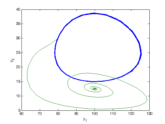
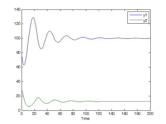
 and
and  are the prey and predators. These are ordinary differential equations that are straightforward to solve.
 , we can arrive at a new set of delay differential equations:

 depends on the value of the solution some time
  , we have to know the history to know the initial derivative is. We use the dde23 function in Matlab to solve this problem.
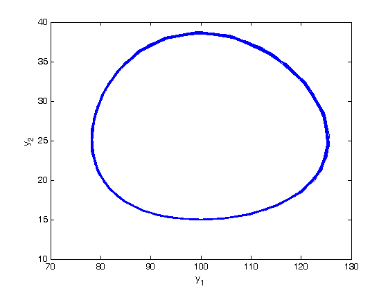
 .
.