Matlab in Chemical Engineering at CMU

Contents

Delay differential equations

http://www.radford.edu/~thompson/webddes/tutorial.pdf (Problem 1 on page 32).

A model for predator-prey populations is given by:

where and are the prey and predators. These are ordinary differential equations that are straightforward to solve.

If there is a resource limitation on the prey and assuming the birth rate of predators responds to changes in the magnitude of the population y1 of prey and the population y2 of predators only after a time delay , we can arrive at a new set of delay differential equations:

these equations cannot be solved with ordinary ODE solvers, because the value of the solution at any time depends on the value of the solution some time ago. So, even at , we have to know the history to know the initial derivative is. We use the dde23 function in Matlab to solve this problem.

function main

clear all; close all; clc

The non-delay model

We first solve the ordinary model so we can see the impact of adding the delay.

a =0.25;
b= -0.01;
c= -1.00;
d=0.01;

y10 = 80; % initial population of prey
y20 = 30; % initial population of predator
tspan = [0 200]; % time span to integrate over
[t,Y] = ode45(@myode,tspan,[y10 y20]);

y1 = Y(:,1);
y2 = Y(:,2);

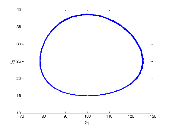
phase portrait of solution

You can see a stable limit cycle (purely oscillatory behavior) in the population of prey and predators.

plot(y1,y2)
xlabel('y_1')
ylabel('y_2')

    function dYdt = myode(t,Y)
        % ordinary model
        y1 = Y(1);
        y2 = Y(2);

        dy1dt = a*y1 + b*y1*y2;
        dy2dt = c*y2 + d*y1*y2;

        dYdt = [dy1dt; dy2dt];
    end

The delay model

Now we solve the model with the delays. We solve this example with a delay of .

lags = [1]; % this is where we specify the vector of taus

% we need a history function that is a column vector giving the value of y1
% and y2 in the past. Here we make these constant values.
     function y = history(t)
         y = [80; 30];
     end

% we define the function for the delay. the Y variable is the same as you
% should be used to from an ordinary differential equation. Z is the values
% of all the delayed variables.
    function  dYdt = ddefun(t,Y,Z)
        m = 200; % additional variable
        y1 = Y(1);
        y2 = Y(2);

        % Z(:,1) = [y1(t - tau_1); y2(t - tau_2)]
        y1_tau1 = Z(1,1);
        y2_tau1 = Z(2,1);

        dy1dt = a*y1*(1-y1/m) + b*y1*y2;
        dy2dt = c*y2 + d*y1_tau1*y2_tau1;

        dYdt = [dy1dt; dy2dt];
    end

now we solve with dde23

sol = dde23(@ddefun,lags,@history,tspan)

y1 = sol.y(1,:); % note the y-solution is a row-wise matrix.
y2 = sol.y(2,:);

sol = 

     solver: 'dde23'
    history: @dde_example1/history
    discont: [0 1 2 3]
          x: [1x127 double]
          y: [2x127 double]
      stats: [1x1 struct]
         yp: [2x127 double]

Add delay solution to the ordinary solution

hold all
plot(y1,y2)

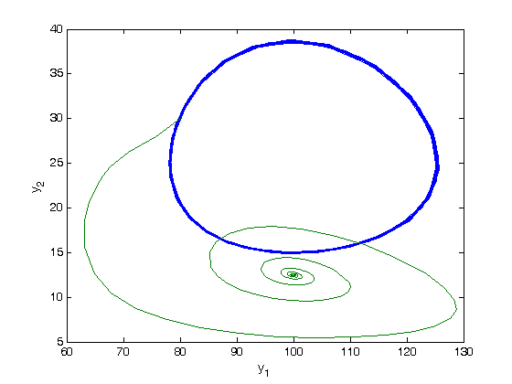
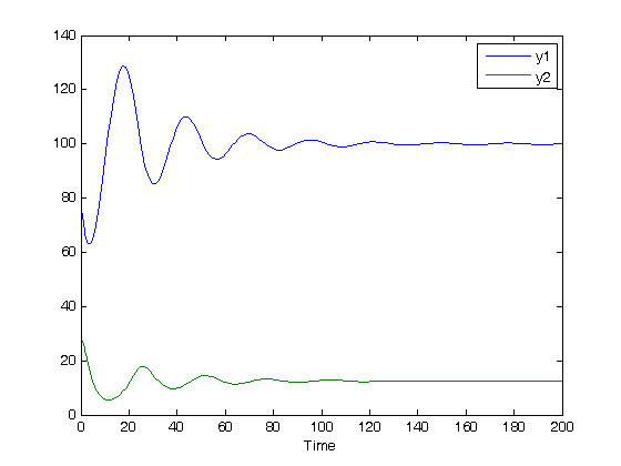
you can see the delay and resource limit significantly affect the solution. Here, it damps the oscillatory behavior, and seems to be leading to steady state population values.

figure
plot(sol.x,y1,sol.x,y2)
xlabel('Time')
legend 'y1' 'y2'

end

% categories: ODEs
% tags: delay differential equation

Published with MATLAB® 7.12