Interacting with graphs with context menus
December 15, 2011 at 02:04 PM | categories: plotting | View Comments
Contents
Interacting with graphs with context menus
John Kitchin
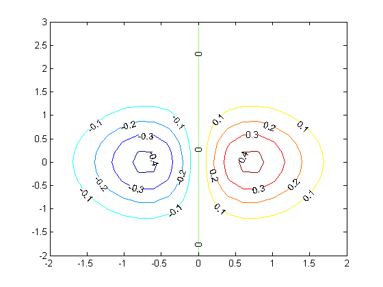
In Post 1489 we saw how to interact with a contour plot using mouse clicks. That is helpful, but limited to a small number of click types, e.g. left or right clicks, double clicks, etc... And it is not entirely intuitive which one to use if you don't know in advance. In Post 1513 , we increased the functionality by adding key presses to display different pieces of information. While that significantly increases what is possible, it is also difficult to remember what keys to press when there are a lot of them!
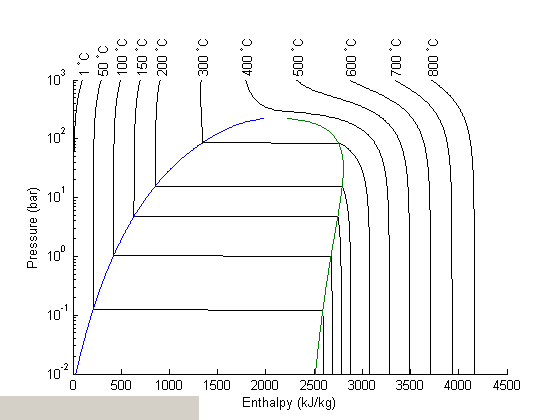
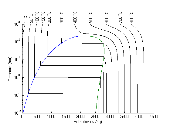
Today we examine how to make a context menu that you access by right-clicking on the graph. After you select a menu option, some code is run to do something helpful. We will examine an enthalpy-pressure diagram for steam, and set up functions so you can select one a few thermodynamic functions to display the relevant thermodynamic property under the mouse cursor.
See the video.
function main
The XSteam module makes it pretty easy to generate figures of the steam tables. Here we make the enthalpy-pressure graph.
clear all; close all
P = logspace(-2,3,500); %bar

temps = [1 50 100 150 200 300 400 500 600 700 800]; % degC
figure; hold all
for Ti=temps
    Hh = @(p) XSteam('h_PT',p,Ti);
    H = arrayfun(Hh,P);
    plot(H,P,'k-')
    % add a text label to each isotherm of the temperature
    text(H(end),P(end),sprintf(' %d ^{\\circ}C',Ti),'rotation',90);
end

% add the saturated liquid line
hsat_l = arrayfun(@(p) XSteam('hL_p',p),P);
plot(hsat_l,P)

% add the saturated vapor line
hsat_v = arrayfun(@(p) XSteam('hV_p',p),P);
plot(hsat_v,P)

xlabel('Enthalpy (kJ/kg)')
ylabel('Pressure (bar)')
set(gca,'YScale','log') % this is the traditional view
% adjust axes position so the temperature labels aren't cutoff.
set(gca,'Position',[0.13 0.11 0.775 0.7])
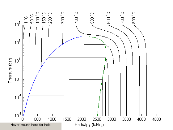
Now we add a textbox to the graph where we will eventually print the thermodynamic properties. We also put a tooltip on the box, which will provide some help if you hold your mouse over it long enough.
textbox_handle = uicontrol('Style','text',...
    'String','Hover mouse here for help',...
     'Position', [0 0 200 25],...
     'TooltipString','Right-click to get a context menu to select a thermodynamic property under the mouse cursor.');

% we will create a simple cursor to show us what point the printed property
% corresponds too
cursor_handle = plot(0,0,'r+');
setup the context menu
hcmenu = uicontextmenu;
Define the context menu items
item1 = uimenu(hcmenu, 'Label', 'H', 'Callback', @hcb1);
item2 = uimenu(hcmenu, 'Label', 'S', 'Callback', @hcb2);
item3 = uimenu(hcmenu, 'Label', 'T', 'Callback', @hcb3);
Now we define the callback functions
    function hcb1(~,~)
        % called when H is selected from the menu
        current_point = get(gca,'Currentpoint');
        H = current_point(1,1);
        P = current_point(1,2);
        set(cursor_handle,'Xdata',H,'Ydata',P)

        % We read H directly from the graph
        str = sprintf('H   = %1.4g kJ/kg', H);
        set(textbox_handle, 'String',str,...
            'FontWeight','bold','FontSize',12)
    end

    function hcb2(~,~)
        % called when S is selected from the menu
        current_point = get(gca,'Currentpoint');
        H = current_point(1,1);
        P = current_point(1,2);
        set(cursor_handle,'Xdata',H,'Ydata',P)

        % To get S, we first need the temperature at the point
        % selected
        T = fzero(@(T) H - XSteam('h_PT',P,T),[1 800]);
        % then we compute the entropy from XSteam
        str = sprintf('S   = %1.4g kJ/kg/K',XSteam('s_PT',P,T));
        set(textbox_handle, 'String',str,...
            'FontWeight','bold','FontSize',12)
    end

    function hcb3(~,~)
        % called when T is selected from the menu
        current_point = get(gca,'Currentpoint');
        H = current_point(1,1);
        P = current_point(1,2);
        set(cursor_handle,'Xdata',H,'Ydata',P)

        % We have to compute the temperature that is consistent with
        % the H,P point selected
        T = fzero(@(T) H - XSteam('h_PT',P,T),[1 800]);
        str = sprintf('T   = %1.4g C',  T);
        set(textbox_handle, 'String',str,...
            'FontWeight','bold','FontSize',12)
    end
set the context menu on the current axes and lines
set(gca,'uicontextmenu',hcmenu)

hlines = findall(gca,'Type','line');
% Attach the context menu to each line
for line = 1:length(hlines)
    set(hlines(line),'uicontextmenu',hcmenu)
end
end

% categories: plotting
% tags: interactive, thermodynamics